So, let me shortly describe Liapunov analysis. Originally equation (1) was developed by Liapunov to investigate stability of nonlinear differential equations. But you can also test chaotic equations as Mario Markus shows. Instead of building the sum of logarithms one can use the product of the derivations, when you are sure that the maximal values will not exceed the maximal values handled by the compiler.

      Equation (2) and (3) have chaotic behaviour when you use them recursively. This means, after choosing a start value (for instance 0.5) for x, you take the result f(x) as the new value for x and so on. In equation (2) variable r must be in the range from nearly 3 to 4, only then chaos appears. To find the best values, you have to experiment a little. Image 1 shows the chaotical behaviour of equation (2) as you can find in many publications (Feigenbaum graph), beneath is a one dimensional Liapunov analysis. Both graphs correspond with each other. Bright yellow is the color of high stability, it becomes dark red for low stability. Blue is the color of chaos.

Feigenbaum graph and Liapunov analysis

To create two dimensional graphs, we have to introduce two further variables, A and B. A corresponds to x and B corresponds to y of the coordinate system. These are the values we need to disturbe the chaotic equation to find out at which point P(x,y) this equation is stable or chaotic. Now we have to insert the results of the derivation of our chaotic equation into equation (1). For each step of the iteration we choose for r either an A-value or a B-value depending on the disturbance sequence (f.i. AAB, ABABBAB and so on). We don't use the first 100 to 500 results of the iteration. They are needed to stabilize the iteration process. After stability is ensured the iteration can be continued until the desired accuracy is obtained (500 to 5000 more iterations). If the modulus of the result lambda is larger than one, the equation shows chaotical behaviour, if it is smaller than one, the equation is stable. Now we only have to choose the right color for our lambda value. If we want to extend the analysis to a further dimension we have to introduce a new variable C (or T for time). The process of iteration is the same as described above.

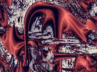
Inspired by the article of Mario Markus I began to write a program (or programme for our English readers) to have the ability to experiment in this world of chaos and order. It was only a short time, when reality crossed my path. I had to find out, that a fast implementation of the algorithms was impossible. You need a software infrastructure to handle the input of these complex data and it is necessary to integrate the graphical output into the graphical environment of the operating system. Furthermore, I found out, that I had to optimize the calculating parts (written in assembler) of the program. Or do you want to wait three weeks for one result? Now this program is optimized (though not totally bug-free) and the user can easily generate new images and experiment with colors and color transition.

Compared to other chaos programs, which usually generate fractals, this program is unique, not only because of the shapes you can create, but also in its way to give the user the possibility to experiment.

 These twodimensional static graphs are really fantastic, but what happens, when we introduce a new dimension, say time? At first we will discover that the calculation time increases dramatically as for each time point we have to calculate one new image. After that, when the calculation phase is finished, we can create a movie of these images. These movies show moving Liapunov shapes, that you barely can describe. To get an impression you can download examples of these movies (Quicktime or AVI) on this internet side. The size of the original movies is 768x576 pixel (video size), the movies you can find here are reduced in their size due to internet use.
 

Why did we create this program, the graphs and movies? Shortly, because we want to inspire ourselves (and, of course, others) to create new forms in industrial design and elsewhere. These images give you a kick to think critically about conventional shapes. In December 1996 we exhibited these images and movies together with modified Liapunov graphs in our university (Braunschweig School of Art).

You can find more infos and images on our internet page:

http://www.hbk-bs.de/Designinformatik/galerie/

For now the sites are in German, but we try our best to offer English pages too. Further information can be obtained by our magazine "Öffnungszeiten" (mainly in German, too) which is available at the Braunschweig School of Art.