q1q14.html

KOS 1110 Computers in Science
Assignment 4 - Questions in Introduction to Maple
Due date Friday, 10-9-2004 5pm

1. Hierarchy of arithmetic operations: Use your own examples (at least three examples and execute them in

maple) to prove which arithmetic operations are carried out first in Maple and if they are of equal priority, in

which directions they are carried?

# The answers obtained were based on the hierarchy of arithmetic which give priority beginning with parentheses ( ),

exponents(^), multiplication(*) and division(/), addition(+) and substraction(-).
# If the operation are equal priority like multiplication and division or addition and substraction, we must solve it from left to

right.

Example 1

> 5*3-6+7/2;

# From the equation, multiplication (*) and division (/) need to be solved first, followed by substraction (-) and addition

(+).The operation was carried out from left to right.

Example 2

> 5*8/4-10+13;

# From the equation, multiplication (*) and division (/) have the first priority compared to others and it is followed by

substraction (-) and addition (+). The operation was carried out from left to right.

Example 3

> 9-4*3+10;

# From the equation, multiplication (*) operation need to be solved first, followed by substraction (-) and addition (+) and the

operation was carried out from left to right.

2. Using your own examples (one example each and execute them in maple) clearly bring out all the differences

    between the following maple symbols and commands:
   a) ; and :
    b) = and :=
    c) ? and ???
    d) expression and function
    e) sum and add

a) ; and :

Example

> restart;

> 2+3-4*5;

> 2+3-4*5:

# (;) and (:) are to execute the commands but the differences between them is ( ;) can display the execution result but if we

use (:) , the result will not display.

b) = and :=

Example

> restart;

> a1:=4*x+2*y-3;

> a1=4*x+2*y-3;

# (=) and (:=) are use to assign the statement.

If we use (:=), the variable which is in this example having a value of the expression. But, if we use (=), the result will assign

to the x. So that the x will have same value of the expression.

c) ? and ???

Example

> restart;

> ?Vector

> ???Vector

# ? - When we execute, we get the general explanation about that topic.

# ??? - When we execute,we get specific explanation of the topic including the examples section( if any) and all other

contracted.

d) expression and function

Example

Function

> restart;

> f:=x->2*x^2-5*x;

# Function represent a function call or application of a procedures to arguments.In this expression,we refer the entire

expression f(x) as being of the type, while the expression f is typically not itself of typefunction. The operands of a function

expression are the arguments.

Expression

> f:=2*x^2-5*x;

# Expression is only represent the arguments.

e) sum and add

Example

Sum

> restart;

> Sum (k/(2*k+1), k=1..infinity)=sum (k/(2*k+1), k=1..infinity);

# The sum command is for symbolic summation. It is used to compute a formula for an indefinite or definite sum.If Maple

cannot compute a closed form, Maple returns the sum unevaluated.

Add

> add(k/(2*k+1),k=1..10);

# To add affinite sequence of values, rather than compute a formula, use the add command.

3. Use of Help facilties in Maple: Use the help commands in Maple and explain the use of three Maple commands

(not discussed in the class) with your own examples.

a) Slope

student[slope] - To compute the slope of a line

      Calling Sequence
     slope(equation)
     slope(equation, y, x)
     slope(equation, y(x))
     slope(p1, p2)

    Parameters
     equation - equation of a line
     y,x      - (optional in most cases) dependent and independent variables
     p1,p2    - two 2-dimensional points (such as [a, b] and [c, d])

Description
· The function slope will compute the slope of a line determined by two points, or by an equation.
· If equation is of the form y = f(x), then the dependent variable is taken to be y, and the independent variable to be x

. Ambiguity caused by three or more unknowns or by the use of a different form of equation is resolved by providing two

additional arguments, y and x, the names of the dependent and independent variables, respectively.
· The command with(student,slope) allows the use of the abbreviated form of this command.

Examples

> restart;

> with(student):
slope(y = 2*x+1);

> slope(y = a*x+1, y, x);

> slope(3*y+5 = x-1, x, y);

> slope(3*y+5 = x-1, x(y));

b) Statistics

       stats[transform, frequency] - Frequency of Each Data Item
      Calling Sequence
     stats[transform, frequency](data)
     transform[frequency](data)
     Parameters
     data - statistical list
    Description
   · The function frequency of the subpackage stats[transform, ...] replaces each data point of data by its frequency or weight.

· The order of the data items is not changed.
· Statistical data items in a list have a weight, obtained using transform[frequency] and a value, obtained using

transform[statvalue]. One can obtained the total frequency, or total weight, using describe[count]. All frequencies in a

     statistical data list can be changed, proportionally, using the transform[scaleweight].
   · The command with(stats[describe],frequency) allows the use of the abbreviated form of this command.

     Examples

> restart;

> with(stats):
transform[frequency]([6]);

> transform[frequency]([Weight(6,7)]);

> transform[frequency]([6..7]);

> data:=[Weight(6,13),missing, 7, Weight(16..16,6), 19..21];

> transform[frequency](data);

c) bernoulli

    - compute Bernoulli numbers and polynomials
     Calling Sequence
     bernoulli(n, x)
    Parameters
     n      - non-negative integer
     x      - (optional) expression
    Description
   · The bernoulli(n) function computes the nth Bernoulli number. Bernoulli numbers come from the coefficients in the Taylor

      expansion of x/(e^x - 1).
  · The bernoulli(n, x) function computes the nth Bernoulli number, or the nth Bernoulli polynomial, in the expression x.
    The nth Bernoulli number is defined as bernoulli(n,0).
    The nth Bernoulli polynomial is defined by the exponential generating function:
      t*exp(x*t)/(exp(t)-1) = sum( bernoulli(n,x)/n!*t^n, n=0..infinity ) .

Examples

> restart;

> bernoulli(3);

> bernoulli(3,x);

> bernoulli(3,1/2);

4. Use of units and Scientific Constants: Select any three problems involving different types of units from your

textbooks and carry out the complete calculations including the units using Maple. State the problem fully and

comment whether Maple gives the correct final answer along with appropriate units. (Refer the examples

discussed in the class)

a) Decay activity for a sample of iodine-131.

The expression for the activity is defined as A where A0 is the initial activity, is the mean lifetime of the isotope and and the t

is the elapsed time.

> restart;

> with(ScientificConstants);

> A:=A0*exp(-lambda*t);

The mean lifetime is related to the halflife by = 0.693/H

> lambda:= 0.693/evalf(Element(I[131],halflife));

Plot with A0=1.

> A0:=1;

> plot(A, t=0..6e6, labels=["time(s)","Activity"]);

b) What is the energy of an electron, E?

> restart;
with(Units);

> mass:=9.11e-31 * kg;

> c:=3.00e8 *m/s;

> E:=mass * c^2;

c) Given capacitance and inductance, find the resistance in microohms.

> restart;

> with(Units[Natural]);

Warning, the assigned name polar now has a global binding

Warning, these protected names have been redefined and unprotected: *, +, -, /, <, <=, <>, =, Im, Re, ^, abs, add, arccos, arccosh, arccot, arccoth, arccsc, arccsch, arcsec, arcsech, arcsin, arcsinh, arctan, arctanh, argument, ceil, collect, combine, conjugate, convert, cos, cosh, cot, coth, csc, csch, csgn, diff, eval, evalc, evalr, exp, expand, factor, floor, frac, int, ln, log, log10, max, min, mul, normal, root, round, sec, sech, seq, shake, signum, simplify, sin, sinh, sqrt, surd, tan, tanh, trunc, type, verify

>

> resistance:=sqrt(inductance/capacitance);

> eval(resistance,[inductance=124.*nH,capacitance=3.52*uF]);

> evalf(%);

> convert(%,units,uOmega);

5. Find out the dimensions of three different physical properties using Maple.

> restart;

a)acceleration

> with (Units);

> GetDimension(acceleration);

b) momentum

> GetDimension(momentum);

c) energy

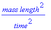
> GetDimension(energy);

6. Calculate the volume occupied by 1 kg of mercury at 25°C.

> restart;

> with(ScientificConstants):

> GetElement (Hg);

> density:=13.5336*g/cm^3;

> mass:=1*kg;

> convert(1,units,kg,g);

> mass:=%;

> volume:=mass/density;

7. Use Maple to calculate the number of water molecules in 1 g of liquid water.

> restart;with(ScientificConstants):

> GetElements:

> 2*Element(H,atomicweight)+Element(O,atomicweight):

> evalf(%);

> convert(%,units,kg,amu);

> 1./%;

> %*evalf(Constant(N['A']));

8. What is computer algebra system and what are its advantages?

# Computer Algebra System or Symbolic Computation is the computation with symbols representing mathematical objects

including :-

a) integers,real and complex numbers

b) polynomials

c) derivatives and integrals

d) system of equation, series expansion of function

# Advantages

a) To obtain closed and exact form of solutions

b) Build thousands of function

c) Greatest option for simplifying expressions

9. Determine whether is linear or not ? (Hint: solve for y and comment)

> solve ({(y+8)/(x-2)=(x+6)},y);

${y = -20+x^2+4*x}$

#Comment : Since there is x power of 2 , it determines that this function is not linear function but it is a quadratic function.

10. Show that z=1, y=2, x=3 are the solutions for x+2y-3z = 4. (Hint: use subs )

> restart;

> A:=x+2*y-3*z=4;

> subs(x=3,A);

> subs(y=2,%);

> subs(z=1,%);

# Proven

11. a) Solve the equations: x - y = -3 and x + 2y = 3. Plot these equations in the same graph. Do these graphs

cross each other? What is the meaning of the point of intersection?

> restart;

> e1:=x-y=-3;

> e2:=x+2*y=3;

> solve({x-y=-3},y);

> solve({x+2*y=3},y);

> plot({x+3,(-x/2)+(3/2)},x=-3..3);

# These graph cross each other at coordinate (-1,2). Intersection point is the point at which graph cross each other.We also

can find the point of intersection between two line by using this command:

> solve({e1,e2},{x,y});

b) Plot the equations: y = -x - 3 and y = -x + 2. From the graphs what can you say about the existence of solutions

for this set of equation?

> restart;

> y:=-x-3;

> y:=-x+2;

> plot({-x-3,-x+2},x=-infinity..infinity);

# There is only one solution since both equation are linear and parallel to each other due to similar slopes.

c) Plot the equations: x + y = 1 and 2x + 2y = 2. From the graphs what can you say about the existence of

solutions for this set of equation?

> restart;

> e3:=x+y=1;

> e4:=2*x+2*y=2;

> solve({x+y=1},y);

> solve({2*x+2*y=2},y);

> plot({-x+1,-x+1},x=-3..3);

# Both equations are give the same set of point.

12. Solve the equations: 2x + y - 2z = 8, 3x + 2y - 4z = 15 and 5x + 4y - z = 1 .

> e5:=2*x+y-2*z=8;

> e6:=3*x+2*y-4*z=15;

> e7:=5*x+4*y-z=1;

> solve({e5,e6,e7},{x,y,z});

13. Write any equation of your own and expand it using Maple. Factorize and simply the result and show that it

gives back the starting equation.

Expand

> restart;

> e8:=(x+3)/2*(x+2*y)/6*(5*x-3*y)/4*(3*y+x)/3;

> expand(%);

Simplify

> simplify(%);

Factorize

> factor(%);

14. Write any equation in with three variables (x, y and z) and solve it using Maple.

> e9:=4*x+5*y-z=40;

> e10:=2*x-y+3*z=-18;

> e11:=x-2*y+4*z=-30;

> solve({e9,e10,e11},{x,y,z});