Contouring Implicit Surfaces
Principles and Practice

by Ronen Tzur (email).

Introduction

A sample implementation is provided for two contouring algorithms: the classic Marching Cubes and the newer Dual Contouring.

Download the zip file containing this page and the sample implementation.

Download a zip file containing pre-compiled binaries.

Implicit Surfaces

Consider the field function for a sphere. It is f(x,y,z) = x² + y² + z² - R² where R is the radius of the sphere. For a point lying exactly on the contour of the sphere--that is, at a distance of R² from its center--the function evaluates to zero. For a point lying outside the sphere, at a distance that is greater than R², the function evaluates to a positive result. And finally, for a point lying inside the sphere, the function evaluates to a negative result.

This representation of volumes in three-dimensional space is very compact and precise. To explicitly describe the sphere from the example above would require specifying a list of points and polygons that make up an approximation of the contour of a sphere. An implicit representation also allows for precise CSG (constructive solid geometry) operations to occur in the domain of the function. To perform such an operation on an explicitly-represented contour would first require figuring out what the actual volume is.

Explicitly-represented contours can be rendered much faster than implicit volumes, as the polygons are already known and can be easily drawn on the screen, often by sending them to a graphics card that is designed to render polygons. To render an implicit surface this way, however, it is first required to compute the polygonal approximation of its contour.

Expressing Implicit Surfaces in the Sample Implementation

An implicit surface is defined by a derivated of the class Isosurface (in files threed/isosurface.*). This class is the interface for implementing the field function d = f(x,y,z) discussed above, by providing a pure virtual function Isosurface::fDensity that computes the field function. To gain better performance, fDensity can compute any number of points, starting at a point specified by three parameters (x0,y0,z0) and progressing towards the +z axis by a delta specified by the parameter dz.

As an example, an implementation of the field function of a sphere using Isosurface would look like this:

class SphereIsosurface : public Isosurface
{
public:
	SphereIsosurface(float rad) : _radius(rad)
	{
		Vector center;	// (0,0,0)
		Vector v1 = center - _radius;
		Vector v2 = center + _radius;
		Isosurface::addBoundingBox(BoundingBox(v1, v2));
	}

	void SphereIsosurface::fDensity(
		float x0, float y0, float z0,
		float dz, int num_points, float *densities)
	{
		for (int i = 0; i < num_points; ++i) {
			float sqr_dist = x0 * x0 + y0 * y0 + z0 * z0;
			float sqr_rad = _radius * _radius;
			float d = sqr_dist - sqr_rad;
			densities[i] = d;

			z0 += dz;
		}
	}

protected:
	float _radius;
};

Note how the constructor of SphereIsosurface computes an axis-aligned bounding box containing the sphere and reports it using Isosurface::addBoundingBox. Generally speaking, it is not easy to figure out the bounding box just by looking at the field function. A few algorithms have been proposed that address this problem, but they are not perfect: for example, they may not work correctly when the field function describes volumes that are not connected. (But see [7], [8] for more information.) In many cases Isosurface is derived to implement solid primitives, such as a sphere, a box, or a torus, whose bouding box can be easily computed. Therefore I find it reasonable to expect the implementation of an Isosurface to report its own bounding box.

The implementation of Isosurface also permits transformation of the volume. The class Matrix (in files threed/matrix.*) implements an 4x4 transformation matrix. Such a matrix can cause any combination of translation, rotation, scaling and shearing operations to occur on a point (or an object made up of a collection of points) in 3D space. The Matrix class is also compatible with the way OpenGL deals with matrices. The class Transform (in files threed/transform.*), that inherits Matrix without adding any new data members, has a function Transform::glMultMatrix which is simply a wrapper around the OpenGL function glMultMatrixf.

A transformation matrix can be applied to the implicit surface using Isosurface::setTransform(). Now consider a sphere of radius 1, that has been translated on the x axis and is now centered at (‑5,0,0). Evaluating the field function for the point at (0,0,0) should return a result indicating the point is outside the volume. In this case SphereIsosurface::fDensity() as presented above will evaluate to an incorrect result, as it does not take the translation into account. But the definition can be easily revised to take any kind of transformation into account:

	void SphereIsosurface::fDensity(
		float x0, float y0, float z0,
		float dz, int num_points, float *densities)
	{
		for (int i = 0; i < num_points; ++i) {
			float xt, yt, zt;
			inverted_matrix.transform(x0, y0, z0, &xt, &yt, &zt);

			float sqr_dist = xt * xt + yt * yt + zt * zt;
			float sqr_rad = _radius * _radius;
			float d = sqr_dist - sqr_rad;
			densities[i] = d;

			z0 += dz;
		}
	}

The revised version first transforms the specified point given by (x0,y0,z0) by the inverted matrix of the transformation applied to the implicit surface. When no transformation has been applied, the transformation matrix is the identity matrix, and so is its inverse, in effect resulting in xt=x0, yt=y0, zt=z0. But to revisit the last example where a sphere is translated by (‑5,0,0), the inverted matrix would translate the point by (+5,0,0), resulting in xt=(x0+5), yt=y0, zt=z0. Thus evaluating the field function at (0,0,0) would correctly return a result indicating the point is outside the volume, while evaluating the point at (-5,0,0) would correctly return a result indicating the point is inside the volume.

Marching Cubes

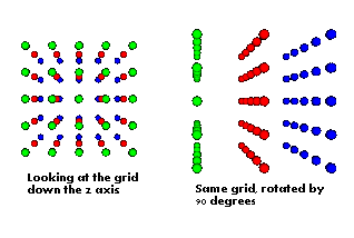
The following illustrations show a grid of size 5x5x3, and an outline of a single grid cube.

This is only an overview of Marching Cubes and far from a comprehensive description. See [3] for a much more in-depth discussion, including a sample implementation of the algorithm. My own implemention is described in the following section.

An Implementation of Marching Cubes

The algorithm is implemented in function IsoMesher_MC::createMesh(), where first an axis-aligned bounding box is computed. The bounding box is computed in the Isosurface itself by the function Isosurface::getBoundingBox() which takes into account any transformations applied on the implicit surface, and also computes the inverted transformation matrix for use by Isosurface::fDensity(). Once the bounding box is known, the number of cubes it contains in each of the three axes x, y and z is computed by a simple division by the size of the cube:

	xsize = ( boundingBox.vmax().x() - boundingBox.vmin().x() ) / cubeSize.x();
	ysize = ( boundingBox.vmax().y() - boundingBox.vmin().y() ) / cubeSize.y();
	zsize = ( boundingBox.vmax().z() - boundingBox.vmin().z() ) / cubeSize.z();

IsoMesher_MC::createMesh() examines the grid in rows. A row is a slice of grid points (not voxels) all having the same y coordinate, and is made up of two two-dimensional arrays: points[xsize][zsize] which holds the (x,y,z) location of the grid point, and densities[xsize][zsize] which holds the result of invoking Isosurface::fDensity() on each of the points. Two rows of grid points describe a single row of grid cubes, as each cube is bound by eight grid points.

Computing a row (as performed by IsoMesher_MC::computeRow()) means initializing the points[][] array and evaluating the field function for each point. To accomplish this, computeRow() has to know the bottom left near coordinate of the row: this is essentially the minimum coordinate of the bounding box, incremented along the y axis as the algorithm progresses throughout the rows.

void IsoMesher_MC::computeRow(const Vector &vRow) {
	float x0 = vRow.x();	// get the bottom left near
	float y0 = vRow.y();	//    coordinate for the
	float z0 = vRow.z();	//    current row of points
	float dx = cubeSize.x();
	float dz = cubeSize.z();

	for (x = 0; x < xsize; ++x) {

		// initialize the points structure
		for (z = 0; z < zsize; ++z)
			points[x][z] = Vector(x0 + x * dx,   y0,   z0 + z * dz);

		// evaluate the points (x,y0,zmin) through (x,y0,zmax)
		isosurface->fDensity(x0 + x * dx, y0, z0, dz, zsize, densities[x]);
	}
}

The function createMesh() uses computeRow() to compute the first grid row at the bottom of the grid, then starts a loop to process each of the subsequent rows from the next-to-bottom row towards the topmost row. For each such subsequent row, it invokes computeRow() to compute it, then calls IsoMesher_MC::marchCubes() to examine the row of grid cubes bound by the two adjacent rows of grid points.

IsoMesher_MC::marchCubes() processes each cube in an x-major, z-minor order. That is, it marches over the x axis of the grid from left to right, and for each x coordinate it marches over the z axis from near to far. Each cube is processed separately: no information that came to be known by processing one cube is needed for processing any other cube. This means than an implementation of the Marching Cubes algorithm can be easily parallelized for multiprocessor environments.

For each cube, the results of the evaluation of the field function for the eight grid points at the corners of the cube are examined. An 8-bit mask is initialized to zero, and each corner is associated with a specific bit position. If the result of the field function for a corner is negative, that is, if the grid point is inside the volume, then the associated bit in the mask is set to 1. This mask describes the relationship of the grid cube with the contour of the implicit surface. The mask is all zeros (0x00) or all ones (0xFF) if the cube is entirely outside or entirely inside the volume, respectively. Any other mask value indicates that some of the corners are inside the volume while others are outside it, and this means the cube intersects the contour in some way and polygons need to be generated.

A cube made of eight corners has 12-edges, any of which can interest the contour. A special table, the edge table, which has 256 entries and is indexed by the bitmask, indicates, using a 12-bit mask, exactly which edges interesect the contour. As each corner was associated with a bit position in the 8-bit mask, so each edge is associated with a bit position in the 12-bit mask. Therefore the bit positions associated with each corner and each edge must be consistent with the values in the edge table. My implementation uses an order similar (but not identical) to the one in [3].

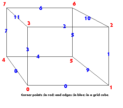
x,y,z denote the bottom left near corner of the cube being processed. corner 0 is at (x, y, z ) corner 1 is at (x+1, y, z ) corner 2 is at (x+1, y+1, z ) corner 3 is at (x, y+1, z ) corner 4 is at (x, y, z+1) corner 5 is at (x+1 y, z+1) corner 6 is at (x+1, y+1, z+1) corner 7 is at (x, y+1, z+1) edge 0 is between corners 0 and 1 edge 1 is between corners 1 and 2 edge 2 is between corners 2 and 3 edge 3 is between corners 3 and 0 edge 4 is between corners 4 and 5 edge 5 is between corners 5 and 6 edge 6 is between corners 6 and 7 edge 7 is between corners 7 and 4 edge 8 is between corners 0 and 4 edge 9 is between corners 1 and 5 edge 10 is between corners 2 and 6 edge 11 is between corners 3 and 7

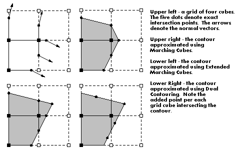
The edge table indicates which edges intersect the contour, but the exact intersection point can lie anywhere on that edge. For instance, if edge table indicates an intersection along edge 2, the exact intersection point lies somewhere on the horizontal line segment that has corners 2 and 3 as its endpoints. There are numerous ways to determine the exact intersection point. The most simplistic approach is to linearly interpolate the position using the results of the field function. (Again, see [3].) While very easy to implement, linear interpolation assumes the field function is continuous. While this may be true for a sphere, it is hardly the general case. Consider the field function for a box:

f(x,y,z) = max(x2 - Rx2,  max(y2 - Ry2, z2 - Rz2))

Iterative evaluation of this function for points that are nearby each other generally returns a smooth progression of values, except at the corners of the box where the use of max causes an abrupt switch from one axis to another. Another case is a volume that is the result of CSG operations on other volumes, which means it is composed of any number of independant field functions. In these cases, employing linearly interpolation to compute the exact intersection point will yield incorrect results.

A far better choice for finding the exact intersection point is the midpoint (sometimes called bisection) algorithm for root solving. [9] According to the midpoint algorithm, the field function is evaluated for the middle point between the two endpoints, and the result is examined. If the result is zero, the exact intersection point was found. Otherwise, the midpoint replaces the endpoint for which the evaluation of the field function has the same sign, and the algorithm re-iterates. In this way the midpoint algorithm iteratively halves the line segment until it finds the line segment whose middle point intersects the contour.

Another choice is the false position algorithm for root solving [9]. It is a combination of both linear interpolation and the midpoint algorithm. Unlike simple linear interpolation, false position finds the exact intersection point even if the field function is not continuous. In terms of performance--the number of iterations made before finding the intersection point--it is no worse than the midpoint algorithm, and usually better. Thus it makes sense to use it as the algorithm of choice for finding the exact intersection point.

Both midpoint and false position algorithms are implemented by class IsoMesher (in files threed/isomesher.*) in the functions IsoMesher::intersect_xaxis(), IsoMesher::intersect_yaxis() and IsoMesher::intersect_zaxis(). The _xaxis version should be used for finding the intersection point on edges 0, 2, 4 and 6 that have fixed y,z coordinates. The _yaxis version should be used on edges 1, 3, 5, 7 that have fixed x,z coordinates. And the _zaxis version should be used on edges 8, 9, 10, 11 that have fixed x,y coordinates. The implementation is of the midpoint algorithm if the preprocessor symbol BISECTION is defined, or of the false position algorithm if the symbol FALSE_POSITION is defined.

An different approach to finding exact intersection points is presented in the Extending Marching Cubes algorithm [12]. EMC modifies the field function to return not one but three values, where each value measures the distance of the point from the contour of the implicit surface on a distinct axis. It employs linear interpolation to compute the x coordinate of the exact intersection point using only the x component of the result of the field function. Similarly it computes the y coordinate using only the y component, and the z coordinate using only the z component.

Once the intersection points are known, they can be connected to form polygons that approximate the contour. The triangle table, which also has 256 entries and is indexed by the 8-bit mask similarly to how the edge table is indexed, specifies which intersection points to connect, and in what order, so that triangles may be formed.

Finding exact intersections points and connecting them to form triangles is accomplished by the function IsoMesher_MC::generateFaces(), which is invoked by IsoMesher_MC::marchCubes() for each cube that was found to intersect the contour in some way. By the time all cubes have been marched through, a complete polygonal approximation of the contour has been generated, and the process is complete.

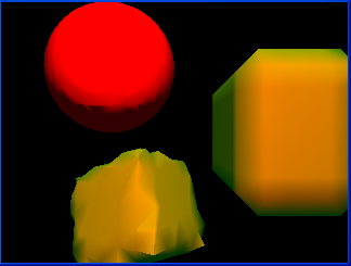
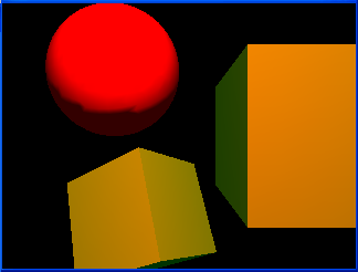
The example program demo1 (in directory demos/) shows how to derive the Isosurface class to define implicit surfaces for a sphere and a box, and how to create a polygonal approximation of an implicit surface using IsoMesher_MC. This is a screenshot of demo1 taken just after invoking it.

When the demo is running, the keyboard and mouse may used to examine the objects in the scene. The gray cursor keys move the viewer around, as well as the gray plus and minus keys. The numeric pad keys 4 and 6 rotate the viewer around the y axis. Clicking the mouse on the object selects it for manipulation. The selected object may rotated using the keys a,d,w,x,q,e, and may be scaled larger or smaller using the keys 1 and 2.

No Sharp Features

Another problem of Marching Cubes--and generally of any implicit surface approximation method that uses a uniform sampling resolution--is that details finer than the resolution of the grid are missed. For instance, consider a box with a small hole carved in it. The polygonal approximation will not exhibit this hole if the hole falls entirely within one grid cube. Approximation errors of this sort may typically be corrected by increasing the resolution of the sampling grid, at the cost of generating far more triangles. This cost can be lowered by using an adaptively-refined grid (or an octree, dividing 3D space into a number of grids of varying resolution) in place of a uniform grid. Some work in this area is presented in [5], [6], [10], [11].

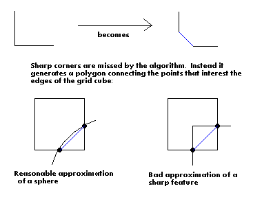
But as noted in [12], refining the sampling resolution (wheather uniformly or adaptively) cannot solve the problem of missing sharp features: "In principle, we could reduce the approximation error of the surface S* extracted from the discretizied field f* by excessively refining the grid cells in the vicinity of the feature. However, the normals of the extracted surface S* will never converge to the normals of S."

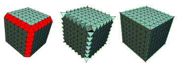
The Extended Marching Cubes algorithm presented in [12] attempts to solve two problems of the classic algorithm. The first is that of computing exact intersection points using linear interpolation, as described in the previous section. The second is that of approximating sharp edges and corners, by examining not only the exact intersection points, but also the normal vector at each point, and using the combination of both to estimate the location of the sharp corner or edge.

The normal vector is a vector perpendicular to some plane. In the context of an implicit surface, the normal vector of some point (x,y,z) in the volume can be approximated as the gradient of the field function in each of the three axes x, y, z.

	nx = f(x + E, y,     z)     - f(x, y, z)
	ny = f(x,     y + E, z)     - f(x, y, z)
	nz = f(x,     y,     z + E) - f(x, y, z)

where E is some small epsilon (eg, 0.001). A plane is defined by a point on the plane and the normal to that point:

	n . p = 0

Consider the case of a grid cube containing the corner point of an implicit box surface. There are three intersection points of the grid cube with the contour. The classic Marching Cubes algorithm connects these points to form the triangle approximating the corner. When the normal vector for each point is known, three planes can be computed. These three planes together form the corner point, and indeed the intersection of three planes is a point.

Given three points P1, P2, P3 and their respective normal vectors N1, N2, N3, solving the following system of linear equations finds the intersection point x.

	N1 . (x - P1) = 0
	N2 . (x - P2) = 0
	N3 . (x - P3) = 0

	[ P1 P1 P1 ]        [ N1 . P1 ]
	[ P2 P2 P2 ]        [ N2 . P2 ]
	[ P3 P3 P3 ]        [ N3 . P3 ]
  	  matrix A            vector B

Now instead of a corner, consider the case of a sharp edge of an implicit box surface. In this case the grid cube will intersect the contour at four points, but these define only two planes. These are the two planes that are on either side of the sharp edge. The intersection of two planes is a line, not a point. In this case the linear system is underdetermined and cannot be solved.

To get around this problem, EMC approximates an exact intersection point using the quadric error function

	E[x] = x - Ni . Pi

This is the least squares solution to the problem. Put simply, the solution of the quadric error function E[x] is the point that is at the same distance from all planes involved. The QEF is best solved using the singular value decomposition (also [13]) of the matrix A from above into the matrices U, D and V, and solving

U D V^T x = b

Using Normals and QEFs in the Sample Implementation

void SphereIsosurface::fNormal(
	float x0, float y0, float z0,
	float *nx, float *ny, float *nz)
{
	float xt, yt, zt;
	inverted_matrix.transform(x0, y0, z0, &xt, &yt, &zt);

	float sqr_dist = xt * xt + yt * yt + zt * zt;
	float sqr_rad = _radius * _radius;
	float d = sqr_dist - sqr_rad;

	sqr_dist = (xt + 0.001f) * (xt + 0.001f) + yt * yt + zt * zt;
	float nx1 = sqr_dist - sqr_rad;

	sqr_dist = xt * xt + (yt + 0.001f) * (yt + 0.001f) + zt * zt;
	float ny1 = sqr_dist - sqr_rad;

	sqr_dist = xt * xt + yt * yt + (zt + 0.001f) * (zt + 0.001f);
	float nz1 = sqr_dist - sqr_rad;

	inverted_matrix.transformNormal(nx1, ny1, nz1, nx, ny, nz);

	normalize_vector(nx, ny, nz);
}

To compute the quadric error function, the polygonizer populates a matrix and a vector similar to the way for solving a linear system of equations as Ax = B. It then invokes the static member function QEF::evaluate() to solve the system using singular value decomposition.

double matrix_A[12][3];
double vector_B[12];
int rows = 0;

for each intersection point {
	// px,py,pz  is the intersection point
	// nx,ny,nz  is the normal vector at that point

	matrix_A[rows][0] = nx;
	matrix_A[rows][1] = ny;
	matrix_A[rows][2] = nz;

	// compute dot product
	vector_B[rows] = (double)(px * nx + py * ny + pz * nz);

	++rows;
}

// solve Ax=B using singular value decomposition

Vector newPoint;
QEF::evaluate(matrix_A, vector_B, rows, &newPoint);

The class QEF (in files threed/qef.*) implements the entire process needed to solve a QEF as a black box usable through QEF::evalute(). The source is documented by there is no practical need to describe the mathematics involved. (The curious reader may refer to [13] for detailed information.)

Dual Contouring

The second drawback has to do with how EMC actually approximates the contour in grid cubes that contain sharp features. The EMC solves the QEF to find point P. It then creates a triangle fan connecting each pair of exact intersection points to the point P. This works well for corners, but for sharp edges the point P is roughly the midpoint of the segment of the edge within the grid cube. (See the illustration below.) The result of this is what appears to be a series of small pyramids along the sharp edges. Therefore EMC requires an additional step of edge flipping, to complete the approximation of the sharp feature.

The Dual Contouring algorithm presented in [14], [15] takes a different approach to using the QEF. It solves the QEF for every grid cube that intersects the contour of the implicit surface, wheather that cube conains sharp features or not. That new point P is assocated with the grid cubes. It approximates the contour by quadrilaterals connecting the P points of four adjacent grid cubes sharing the grid cube edge where an intersection with the contour occurs.

The grid is examined in a bottom-to-top, left-to-right, near-to-far sweeping motion. Therefore for each grid cube, only edges 5, 6, and 10 need to be examined to decide which four adjacent grid cubes participate in the generation of the quad polygon. (The number of edges is the same as with Marching Cubes.) If the reason for only these three edges being important is not immediately clear, the following example should clarify the issue.

If the bottom, left, near grid cube, call it cube A at position (x,y,z), intersects the contour, it can only intersect it on edges 5, 6, or 10. All other edges would definately be on the outside of the implicit surface. If the intersetion is on edge 6, then the three other grid cubes sharing the edge are:
- cube B, immediately to the far side of cube A, at position (x,y,z+1)
- cube C, immediately to the above of cube A, at position (x,y+1,z)
- cube D, immediately to the above and far side of cube A, at position (x,y+1,z+1)
A quad is generated connecting the new points of each of the four adjacent cubes A, B, C, D.

As the algorithm sweeps near-to-far along the grid, the next grid cube to be processed is cube B. It intersects the contour at least on its edge 2, since the grid cube to its near side (that is, cube A) intersects the contour on its edge 6. Cube A's edge 6 is the same as cube B's edge 2. But the quad connecting these two (and two other) grid cubes has already been generated during the processing of cube A.

This logic works the same way if cube A was interesecting the contour on edges 5 or 10. Therefore for any grid cube, examining any edge other than 5, 6, or 10, means re-doing work that was already done for a previous grid cube.

An Implementation of Dual Contouring

The first difference between the two polygonizers is that IsoMesher_DC works with three rows of grid points instead of only two as in IsoMesher_MC. This is due to the fact that Dual Contouring connects four adjacent grid cubes into one quad, and if the intersection is on edges 6 or 10, two of the cubes will be from the row of grid cubes (not grid points) immediately above the row of grid cubes being processed.

IsoMesher_DC also has a notion of a cube structure, where IsoMesher_MC only knows about rows of grid points. For a row of xsize by zsize points, there are (xsize - 1) by (zsize - 1) cubes. Each cube structure keeps its 8-bit mask (same 8-bit mask as in Marching Cubes) and the coordinates computed for its new point.

The process of evaluating the field function (in IsoMesher_DC::computePoints()) is identical to that in IsoMesher_MC. IsoMesher_DC::computeCubes() is similar to IsoMesher_MC::marchCubes() in that is examines the grid cube to see if it intersects the contour, but unlike the Marching Cubes version, it does not generate any polygons. Instead, it calls IsoMesher_DC::generateVertex() to compute the new point, and stores it along with the 8-bit mask in the cube structure.

The process of computing the new point in IsoMesher_DC::generateVertex() is simply computing the exact intersection points as was done in Marching Cubes, and storing these points along with their normals in the matrix A and vector B described above for use with the QEF solver. It then invokes QEF::evaluate() to compute the new point. One thing to note is that it computes the mass point, the average point of all intersection points. The point stored in the vector is really the intersection point minus the mass point. And the mass point is added back into the result of the QEF to produce the new point that is stored in the cube structure. The use of the mass point is needed to guarantee that the computed point will lie within the grid cube even when the system of linear equations is underdetermined.

Once three rows of grid points and two rows of grid cubes have been computed, the next step is to generate quads, accomplished by IsoMesher_DC::generateQuads(). This function examines (xsize - 2) by (zsize - 2) grid cubes of the row of grid cubes. Note that there is no need to examine the very last grid cube because it does not have any neighboring cubes that share its edges 5, 6 or 10. IsoMesher_DC::generateQuads() examines edges 5, 6, and 10 for each cube to see which three adjacent grid cubes to use for the generation of the quad.

Edges 5, 6 and 10 are used to pick the three adjacent grid cubes, but this is not enough to tell the ordering of vertices in the quad. The ordering of vertices is reversed in these three cases:
- for edge 5, if corner 5 is inside the volume (as opposed to corner 6 being inside)
- for edge 6, if corner 7 is inside the volume (as opposed to corner 6 being inside)
- for edge 10, if corner 6 is inside the volume (as oppposed to corner 2 being inside)

This is only important when the graphics subsystem performs backface culling and skips the drawing of polygons that are not facing the viewer. In this case examining the corners guarantees a closed polygonal approximation of the implicit surface.

The example program demo2 (in directory demos/) renders the same image as demo1 using IsoMesher_DC. This is a screenshot of demo2 taken just after invoking it, showing how well Dual Contouring performs for curved surfaces as well as those having sharp features.

Constructive Solid Geometry

In CSG there are generally three ways to combine solid object. The union operation adds or merges any number of solid objects. The intersection operation keeps only those parts of the objects that are overlapping. The difference operation subtracts from the first object the union of all other objects.

The class CsgIsosurface (in files threed/csgisosurface.*) derives Isosurface to implement CSG operations. An instance of CsgIsosurface performs a single CSG operation on its children. The specific operation is set with a call to CsgIsosurface::setCsgMode() with a parameter of CSG_UNION, CSG_INTERSECTION, or CSG_DIFFERENCE. Children are added one at a time using CsgIsosurface::addChild(). The children are any derivative of Isosurface such as the SphereIsosurface or BoxIsosurface or even another instance of CsgIsosurface.

CsgIsosurface::fDensity() invokes Isosurface::fDensity() on each of the children of the CsgIsosurface. But it has to return only one value from this set of values. (Actually it has to store that value in the densities parameter.) For a union operation, if a point is inside at least one implicit surface, it considered inside the combined volume. Therefore the minimal value from set of values is selected. For an intersection operation, all points must be inside, so the maximal value is selected. For a difference operation, which is basically an intersection of the first object with the inverse of all other objects, all but the first value in the set are negated, and the maximal value of this new set is selected.

The example program demo3 (in directory demos/) renders a sphere subtracted from a box using IsoMesher_DC. This is a screenshot of demo3 taken just after invoking it.

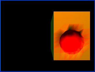
Notice how the different materials merge at the edges of where the CSG operation occurs. The polygonizer does not take materials into consideration, and this can lead to generation of polygons where the color drastically changes between vertices. To separate different colors (or materials) into distinct colors, it is necessary for the polygonizer to treat material changes in the implicit surface the same way as it does the change between inside and outside.

Compiling the Samples

To compile and run the samples, you need to have cygwin installed. Make sure your installation of cygwin contains the OpenGL headers and libraries. You additionally need the SDL library.

Legal Stuff

You may not reprint this article in any form, electronic or otherwise, without expressed consent from the author.

The source code of the sample implementation--that is, all files in the threed and demos directories contained in the zip archive--is hereby put in the public domain. Do with it what you will.

THE AUTHOR MAKES NO REPRESENTATION ABOUT THE SUITABILITY OF THIS SOURCE CODE FOR ANY PURPOSE. IT IS PROVIDED "AS IS" WITHOUT EXPRESS OR IMPLIED WARRANTY OF ANY KIND. THE AUTHOR DISCLAIMS ALL WARRANTIES WITH REGARD TO THIS SOURCE CODE, INCLUDING ALL IMPLIED WARRANTIES OF MERCHANTABILITY AND FITNESS FOR A PARTICULAR PURPOSE. IN NO EVENT SHALL THE AUTHOR BE LIABLE FOR ANY SPECIAL, INDIRECT, INCIDENTAL, OR CONSEQUENTIAL DAMAGES, OR ANY DAMAGES WHATSOEVER RESULTING FROM LOSS OF USE, DATA OR PROFITS, WHETHER IN AN ACTION OF CONTRACT, NEGLIGENCE OR OTHER TORTIOUS ACTION, ARISING OUT OF OR IN CONNECTION WITH THE USE OR PERFORMANCE OF THIS SOURCE CODE.

Have a nice day.

References

[2] Bloomenthal J., Polygonization of Implicit Surfaces, Computer Aided Geometric Design 5, pp 341-356, 1988

[3] Burke P., Polygonising a scalar field (http://astronomy.swin.edu.au/~pbourke/modelling/polygonise/), May 1997

[4] Lorensen W. and Cline H., Marching Cubes: a high resolution 3D surface construction algorithm, Computer Graphics (SIGGRAPH 87 Proceedings), pp 163-169, 1987

[5] Hall, M. and Warren, J., Adaptive Polygonalization of Implicitly Defined Surfaces, IEEE Computer Graphics and Applications, pp 33-42, 1990

[6] Cignoni, P. et al, Reconstruction of Topologically Correct and Adaptive Trilinear Isosurfaces, Computer & Graphics, Vol 24 no 3, pp 399-418, 2000

[7] Witkin A. and Heckbert, P., Using Particles to Sample and Control Implicit Surfaces, Computer Graphics (SIGGRAPH 94 Proceedings), pp 269-278, July 1994

[8] Akkouche S. and Galin E., Adaptive Implicit Surface Polygonization Using Marching Triangles, Computer Graphics Forum, Vol 20 no 2, pp 67-80, June 2001.

[9] Pitman, B. Introduction to Numerical Analysis (http://www.math.buffalo.edu/~pitman/courses/mth437/na/na.html)

[10] Velho, L. Simple and Efficient Polygonization of Implicit Surfaces, Journal of Graphics Tools, Vol 1 no 2, pp 5-24, February 1996

[11] Livnat, Y. et al, A Near Optimal Isosurface Extraction Algorithm Using The Span Space, IEEE Transactions on Visualization and Computer Graphics, 1996

[12] Kobbelt, L. et al, Feature Sensitive Surface Extraction from Volume Data, SIGGRAPH 2001, Computer Graphics Proceedings, Annual Conference Series, pp 57-66, 2001

[13] Golub, G. and Van Loan, C., Matrix Computations, 3rd ed., Baltimore, MD: Johns Hopkins University Press, pp. 70-71 and 73, 1996

[14] Ju, T. et al, Dual Contouring of Hermite Data, ACM Transactions on Computer Graphics (SIGGRAPH 2002 Proceedings), pp 339-346, 2002

[15] Schaefer S. and Warren J. Dual Contouring: The Secret Sauce