BEAUTIFUL UNIVERSE:

TOWARDS RECONSTRUCTING PHYSICS

FROM NEW FIRST PRINCIPLES

 

By Vladimir F. Tamari

4-2-8-C26 Komazawa, Setagaya-ku, Tokyo Japan 154-0012

vladimirtamari@hotmail.com

10 July 2005

 

ABSTRACT

 

A proposal to reconstruct physics from simple physically realistic first principles is outlined using a Beautiful Universe model. Only one type of ‘building block' is used: a spherically-symmetrical charged node spinning with angular momentum in units of Planck’s constant (h).  Rotating nodes become magnetized and self-assemble as a regular face-centered cubic lattice to form the vacuum, radiation and matter. Non-spinning nodes make up dark matter. Three space and one time dimension are derived from the lattice and node interactions.  Mutual repulsion between nodes accounts for the expansion of the universe. A spinning node transfers its angular momentum to adjacent nodes by rotating on an orthogonal axis, thus creating an electromagnetic field with forward momentum. The spin rate of the node receiving the momentum, its ‘density’ determines the rate c_v at which it receives the radiation. In a vacuum c_v is the maximum, c₀ the velocity of light.  Two or more adjacent nodes locked together through a tensegrity of attractive (+ -) and repulsive electrostatic forces form as matter.  The surrounding nodes orient their axes to form magnetic, gravitational or electrostatic fields. The inverse-square law and E=mc₀^2 are derived from the resulting geometry.  Motion of matter is a self-convolution of an energy pattern in the lattice. This links the concepts of Newtonian force and mass with in units of h, whereby a collision causes a Heaviside contraction of an object’s length. Doppler shifts in the signals used by an outside observer to measure the moving object causes a further contraction in the estimated length, similar to the effects of a time dilation. The two effects explain a result of Special Relativity in classical terms. Using the Hamiltonian Analogy and the idea of a node index of refraction n=c_o/c_v General Relativity is reduced to the dynamics of energy transport along streamlines made up of nodes of different spin. Variable velocity along curved streamlines is acceleration and hence gravity. Quantum probability is derived from the electric field of a dipole wave in the lattice. Heisenberg’s uncertainty relations emerge naturally from the resulting geometry. Cosmological inflation, but not a Big-Bang singularity would result from initial conditions of nodes in their closest proximity to each other. The outline of a discrete calculus needed to describe the model’s interactions is presented. Some experiments are proposed to test various aspects of the model.

 

Key words: Physical Theory. Theory of everything. TOE . Special Relativity, General Relativity. Node. Lattice. Quantum Mechanics. Uncertainty relations. Discrete Calculus. Ether, Heaviside. Planck’s Constant. EPR. Expanding Universe. Inflation. Anomaly.

 

1.      THE BEAUTIFUL UNIVERSE (BU) MODEL

 

1.1       THE NEED FOR REALISTIC THEORIES CLOSE TO NATURE

 

             Nature is now complex, but is believed to have evolved systematically over billions of years, following simple processes. This is the lesson of the theories of evolution[1], of fractal equations[2], cross-stitch embroidery[3], digital philosophy[4], and of Wolfram’s book A New Kind of Science[5]: A very simple effect, principle, rule or algorithm applied repeatedly leads to a very rich and complicated outcome.  In their efforts to discover the laws of nature, however, philosophers and physicists in different eras and belonging to different cultures were guided not only by their own thoughts and chance discoveries, but also by the intellectual baggage of their time: the accumulated knowledge , preconceived ideas, and even theological concepts.

            It is no wonder then that present-day physics is a hodge-podge of complicated ideas that do not always work well together, if at all. For example the theory describing gravity on a large scale, General Relativity (GR)[6] and the theory describing atomic and nuclear processes, Quantum Mechanics (QM)[7], speak different ‘languages’ describing what in the end must be the same phenomena. Moreover both (GR) and (QM), although extremely successful in predicting experimental results, both use non-intuitive ideas that seem far from reality. As with the preceding classical physics of Galileo and Newton, these theories describe the behavior of space, mass, time, or gravitation, but give no inkling of what these entities are. A lack of a self-consistent physical model of nature at its most basic level has allowed physicists to accept almost without question some of the more bizarre conclusions of (QM) such as instantaneous interaction at cosmic distances.  This contradicts a basic premise of Special Relativity (SR)[8] that signals cannot travel faster than the speed of light.

 

Such confusion is possible because vastly different mathematical models to describe the same physical phenomena can be derived: even within (QM) itself, Schrödinger’s wave equation[9] was found to be exactly equivalent to a very different mathematical model, Heisenberg’s matrices[10].  But if a model is not ‘true to nature’ its very success distracts from other possibilities, blocking further progress. That happened with Ptolemy’s concept of the Earth staying still while the Sun and the planets rotated around it in complicated circular epicycles[11]. The system ‘worked’ even succeeding in predicting eclipses, because relative to an observer on Earth that is how the planets seemed to move. However it was not until Copernicus[12] put the Sun at the center that Kepler[13] could discover the much simpler elliptical orbits for the planets, paving the way for Newton’s law of gravitation[14] and modern physics.

 

            Similarly, although the concept of flexible spacetime ‘works’ in (SR)  and (GR), and that of probability waves ‘works’ in (QM), they are just mathematical ideas that must be discarded if better models closer to nature can be found. This is more than just a way to seek more elegant theories:  understanding nature at its own level is a necessary step to pave the way for further theoretical, experimental and technological discoveries. The human brain evolved over millions of years in organisms that interacted directly, causally and locally with inanimate nature on a molecular scale[15]. Is it too much to ask now that our understanding of Mother Nature should also be as simple, direct and realistic as possible?

 

1.2       A NEW START

 

There is a widely recognized need to ‘start all over’[16], using the hard-won results of 20^th Century physics, but reconstructing them out of a few basic self-consistent premises.

 

            In the last few decades a great number of papers and books introduced new starting points at various levels of sophistication and completeness: Twistor Theory[17], various theories based on an ether particle[18], Quantum Gravity[19] and many others. String Theory[21] represents such a new start but it creates even more complications with ten or more dimensions using new mathematics, making the theory unlikely to be true to nature in the sense discussed above.

 

The ideas behind Beautiful Universe (BU), the model presented here, derived from my discovery that a classical dipole’s electromagnetic potential field and its streamlines form a miniature united field from which can be derived many of the known phenomena of (SR), (GR), and (QM)[22].  (BU) theory describes a whole universe made up of charged particles spinning as dipoles, (including regions of dark matter where the particles have no spin). In the following sections, the (BU) model will be presented from first principles. In Section 2 an attempt will be made to show that the experimental results, but not the assumptions or all the methods of Newtonian physics, (SR), (GR) and (QM) and related cosmological theories may eventually be derived simply and directly from (BU).  In Section 3 experiments that may prove the correctness of the (BU) approach are proposed. The (BU) presented here is incomplete, and the treatment is qualitative and elementary. The aim is to gain a sure physical understanding of the proposed model’s basic concepts, leaving to future work the necessary but more abstract task of describing it systematically, quantitatively and mathematically.

 

1.3       A NETWORK OF CHARGED NODES CREATES SPACE AND TIME

 

            It is hypothesized that the entire universe is made up of an ordered lattice of identical spherically-symmetric charged nodes that are smaller than the smallest known nuclear particle, but are on a similar scale to it.  This network of nodes creates space itself, so it is meaningless to speak of the shape of an individual node, neither of the material it is made of, or its behavior nor of any space between nodes. Nevertheless to facilitate our understanding, a node can be thought of as being spherical, capable of spinning freely in place around any axis passing through its center. Either at cosmological initial conditions or during the universe’s later development, volumes of nodes rotate and interact with other volumes rotating in an opposite direction (FIG. 1).

 

This cosmic angular momentum is acquired by individual nodes, and can be transmitted to neighboring nodes without friction, but will never disappear, conserving angular momentum locally and in the universe as a whole. Again, we can use the terms of classical physics here only as an analogy, but having like charge, the nodes repulse each other and create an expanding universal space.  It is theorized that individual nodes all over the universe spin in the same direction around their own axis.

 

 

 

 

FIG. 1. An imagined scenario for the creation of spin in nodes. (a) Two volumes of charged particles impinge on each other, as each volume rotates in the opposite directions. Their interaction causes individual nodes to acquire spin.

(b) The resulting volume of spinning magnetized nodes self-assemble to creates an expanding space. There is also the possibility that the nodes exist within other undetected dimensions D (dashed outline).

 

Spin plays a central role in (BU) and both the physical situation and the terms used should be clear.  There is first the ‘rotation’ of vast volumes of nodes without the individual nodes spinning on their axis (FIG. 1).  A dark-matter node is one without spin (FIG. 2a).

 

FIG. 2 the three possible states of nodes (a) basic charged node. (b) Spinning around one axis, with angular momentum in units of Planck’s constant h. (c) Spinning around two axes creates forward momentum (large arrows).

 

 ‘Spin’ is when an individual node rotates around its axis so that it becomes a magnetic dipole (FIG. 2 b) with angular momentum in units of (h) without affecting adjacent nodes.  ‘Forward momentum’ is when the magnetic dipole spins on another axis orthogonal to the dipole axis.  The word ‘forward’ is used because such spin causes adjacent nodes to rotate, as follows:

 

When spinning, a node becomes a magnetic dipole and generates Coulomb-like interactions[23] between neighboring dipoles. In a static field of adjacent spinning nodes the (+ +) and (- -) poles repulse each other until an all the nodes are so oriented that a state of equilibrium is reached, even though each node continues to spin around its own fixed axis.  When a node acquires forward spin, additional angular momentum in multiples of Planck’s constant[24] (h = 6.626068 × 10^-34 m² kg / s) is generated, (FIG. 2c) and this momentum (p) is passed on completely without ‘friction’ and distributed to the immediately adjacent nodes in the forward direction. When this occurs the magnetic dipole axis of the recipient node will twist according to the amount of momentum it received.

 

When two or more spinning nodes in a field are forced to lock in place with opposite poles attracting, (+ -) or (- +) static structures of matter are created (FIG. 3).

 

 

 

FIG. 3 A simple particle forms when two spinning nodes change their orientation and are ‘locked’ because of the attraction of (+ -) poles.  The orientation angles of the node axes,, and their polyhedral arrangements define the possible ‘quantum spin’ states of the particle.

 

This in turn sets the spin orientation and energy of all other surrounding nodes.  It is suggested that the term ‘quantum spin’ be used when referring to spin as it is now used in (QM). ‘Quantum spin’ does not define a rotation around an axis, but the possible symmetries of a particle in space.

 

Everything in (BU), space, energy, radiation, matter is just patterns of nodes rotating in place and forming the universal lattice.  Apart from this rotation around various axes sharing fixed centers,  it is assumed that a node never rolls freely in space, bounces against matter, collides with other nodes like billiard balls, or flows like a grain in shifting sand A vast volume of nodes might conceivably slide, shearing from an adjacent volume, leaving an inhomogeneous ‘fracture’ in the lattice. This will not be considered here, where it will be assumed that node centers are always fixed, and only angular momentum is transferred from one node to its neighbor. 

 

            The (BU) interactions described above may be all the necessary and sufficient premises needed to describe all of the known phenomena of physics at its most basic level.

 

1.4        RADIATION IN VACUUM

 

          Coulomb-like repulsion and attraction between the spinning magnetized nodes and self-assembly create a minimum-energy arrangement of nodes in equilibrium that we know as the vacuum.  All the nodes forming the vacuum have identical spin

 

(1)                    s_o=h       

 

The square-face Kepler packing was recently proven to be the densest packing possible for spheres[25] (FIG. 4), and Gauss proved that the face-centered cubic (FCC) packing is the densest lattice possible[26].  The (FCC) occurs in nature, for example ZnS, or zinc blende, has a face-centered cubic arrangement of sulfide ions with zinc ions in every other tetrahedral hole. An FCC and its tetrahedral components are shown in (FIG. 4).

 

 

 

 

 

 

FIG. 4 Self-assembly of magnetic dipole nodes oriented in the same direction as a Kepler packing. Each unit of the packing forms a cube with a node at each corner, with another node where the cube’s diagonals cross. The smallest regular volume made up of four nodes would be a tetrahedron (shaded).  

 

To maintain this state of minimum energy, the axes of the nodes in vacuum are in static equilibrium and as nearly parallel as possible. On the other hand, there exists the possibility that besides their usual rotation about their spin axis, the axis itself is also rotating about its center, so that all nodes in the universe are in synchronous rotation around two axes at once unless disturbed. Such rotation in unison would prevent the + and – poles of adjacent nodes in vacuum from clumping up because of the attractive Coulomb forces.

 

The cubic symmetries of the node packing are responsible for the three dimensions of space. It is unnecessary here to speculate whether the nodes are set in yet one or more other hidden dimensions, causing their assumed behavior. This possibility, however, would raise the question of the universe having a center, with unequal distance and time scales in radial or tangential directions as shown in Fig. 36  below.

 

Electromagnetic waves are created when an arrangement of matter loses equilibrium and forward angular momentum is released successively from node to neighboring node in a falling-domino effect.  A given node now possesses spin s_v in integral multiples of (h).

 

(2)                    s_v= j s_o =jh        (j=1,2,3…)­

 

creating a magnetic effect and capable of forward momentum. In a process similar to magnetic induction, each node transfers all of its momentum to the handful of nodes in ‘front’ of it in the lattice dividing its energy between them as in (FIG. 5).

FIG. 5 Forward momentum (large arrows) is transferred from node A to neighboring nodes. B gains most of the momentum, since it shares the plane (shaded) in which contains both of their spin axes. This gain in angular momentum causes B to twist by an angle . Lesser twisting is experienced by node D whose axis is normal to that of the forward momentum of A. Other nodes such as C in diagonal directions from A, twist at even lesser angles.

 

This transfer is complete and lossless, and when two or more pulses arrive at a given node simultaneously, they superpose and interfere, adding their momentum linearly as vectors (FIG. 6).

 

 

 

 

 

 

FIG. 6. Two modes contributing their momentums to the adjoining node to the right. The momentums add vectorially and interfere according to their phases.

All the momentum of the donor node is passed to the adjacent nodes and propagates forward and outwards, spreading from node to node within the lattice (FIG. 7).  How much momentum each node receives and in what direction requires careful analysis: a node directly aligned with the momentum vector will get more forward momentum than that located diagonally to the side.  As a result of these interactions the nodes in free space acquire different amounts of spin and align themselves in various orientations. The resulting fields will have equipotential surfaces _constant where  the change of angle between neighboring nodes is constant.  Normal to _constant , the field streamlines are the paths along which the energy of the field is initially propagated. If the field is in equilibrium the nodes settle in unchanging orientation, and  indicate the field curvature. If momentum is continually being transferred a radiation field is the result as in (FIG. 7).

 

As each charged node spins it creates its own magnetic B and electric E fields within itself. These effects only appear when the spinning behavior of adjoining nodes is affected.  The use of the B and E terms here is assumed ad hoc, and is only justified by what we know of the macroscopic behavior of radiation, and not from basic principles. On the scale of the nodes, it is not possible to speak of a continuous streamline line joining three or more congruent nodes, because of the step-like geometry of the packing.  However, along a line of successive nodes the spin axis changes direction in a harmonic motion similar to that of (FIG. 8)

 

 

FIG. 7.  Fields in (BU) can be in equilibrium (a), (b), (c), or time varying radiation fields (d). In all cases equipotential surfaces ( ) are where node-to-node orientation  is constant. Streamlines (S) are normal to (). (d) The nodes in a radiation field transfer angular momentum along (S) so that nodes on successive () have different phase angles  at various times t0,t1,t2,…

 

 

FIG. 8.  Nodes transferring their spin and forward momentum as part of an electromagnetic pulse radiating along a streamline S in the z direction. The Magnetic (B) component of the nodes’ rotation creates the electric field and Electric components (E) create the electric field. Any component of the rotation in the xy plane creates polarization.  The strength of (E) and (B), hence the intensity, is determined by the node spin. The colors are a graphic aid and have no physical significance.

 

 

1.5       VELOCITY OF INTERACTION, SPACE AND TIME

 

There is no time dimension presupposed in (BU) theory, only successive ‘instantaneous’ local states of the universe. Spatial directions, i.e. dimensions, do not have an inherent reality either, but result from the geometry of the node packing. Distances exist because signals traverse different numbers of nodes in succession. However for convenience, and to keep track of the various states of a local volume of space involving many nodes, a minimum unit of time t₀ is defined using a hypothetical separation d₀ between nodes, whereby angular momentum in a vacuum free from and far away from matter, is transferred from node to node with a velocity c₀.  This is the maximum speed of light c in vacuum c= c_o = 2.99792458 times 10^8 meters per second.

 

(3)                    c_o = d_o / t_o

 

If the nodes to which the forward momentum is transferred have a spin s₁>s₀, then the pulse will be delayed, and will travel over a smaller number of nodes, i.e. a distance, as compared to one in vacuum, where nodes have spin s_o  (FIG. 9).

 

 

 

 

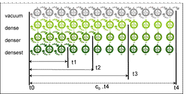
FIG. 9 radiation travels at a maximum speed of c₀ in a vacuum free of matter, but at lesser speeds where the potential is higher, i.e. the nodes are denser, spinning at a higher than the vacuum rate s_o

 

             Assuming that the relationship between the velocity of transfer depends linearly on the inverse of the spin of the node receiving the momentum and its orientation,  

(4)                   

           

 where M is a geometrical inclination factor depending on the direction in the lattice between the donor node and the node receiving the momentum as will be explained in section 2.2 below. When the direction is orthogonal to the faces of the FCC M=1, and √3 when it is diagonal. The pulse velocity c_{v <} c_o is measured by the distance it travels compared to an adjacent pulse traveling in vacuum.  Straight-line distances are measured by the number j of nodes a signal traverses:

 

(5)                    d_o=j Md_o                     (j= 1,2,3…)

 

A local index of refraction of space n or its inverse  can now be defined:

(6)                   

 

Angular momentum spreads as energy in the lattice as light would in a transparent medium having a variable index of refraction such as the atmosphere with variable density gradients[27], or in a gradient index GRIN lens[28] as in (FIG. 10).

 

FIG. 10 (a) A light wave radiates in vacuum of index of refraction n_o=1 (b) In an inhomogeneous potential field of variable index of refraction the wave is distorted accordingly by refraction.  Particles (not shown) having the same momentum and traveling in the same media would be similarly ‘refracted’ (large arrows).

 

 

1.6       MATTER

 

While radiation is a dynamic spreading group pattern of momentum passed from node to node, matter at rest is a pattern of nodes with their axes locked in position or rotating in place, the result of mutual attraction and repulsion in static or dynamic equilibrium within the lattice.

 

The axes of locked nodes are oriented along a direction defined by two angles according to some chosen coordinate system. The nodes form edges or vertices of 3-dimensional polyhedral structures, the simplest of which is a tetrahedron. For example the two nodes of FIG. 3 have their axes aligned along the same line. Here the   twist in the node polarity defines the quantum spin (qs) of the particle. (qs) describes geometrical orientations and symmetries, and not spin (s) in the sense of rotation used above.  The 3D geometry allows larger pieces of matter, existing within larger polyhedra, to have many more possible orientations. A node cannot change its axis without affecting those of the surrounding nodes with the locked nodes both within matter and in the surrounding field up to infinity. To do so requires a lot of energy, as illustrated  in the hypothetical case of a unit particle made up of two adjacent nodes locked as a particle as in (FIG. 11).

 

A hypothetical ‘explosion’ of two-node matter in a vacuum lattice is imagined. At time t= t₀ all nodes except node A are assumed to be oriented in the same upwards direction and having unit spin (s). Due to some influx of momentum from the left, (not shown) A untwists, its axis of orientation and rotates by 180° (π radians) suddenly, while its twin remains fixed. This twist constitutes forward momentum, but its direction is not radially outwards in the plane of the spin axis, but normal to that axis. The adjoining nodes adjust their orientation accordingly, and the twist-induced momentum is transferred as a pulse radiating as a hemispherical shell at a velocity c_o .The number of nodes J on any hemisphere of radius (r) is J=a_n2 π r² where (a_n) is the average number of nodes per unit area of a large sphere.  In one second the shell reaches the nodes aligned on hemisphere H of radius c₀ (the distance energy travels in vacuum in one second) so that J_c0= a_n 2π c₀². In this one second each of the J nodes has twisted by π or less, according to its position on H the total change. A full twist in one second represents a gain of angular momentum of (h).

 

 

FIG. 11 A hypothetical example of matter releasing its locked energy. (a) Node A in vacuum is locked with another node to form a particle. (b) Forces (not shown here) force Node A to rotate by π about an axis normal to its spin axis, acquiring state A’. (c) The released momentum from A causes a twisting effect to be transferred radially from node to adjacent nodes, and after one second the effect reaches nodes such as B, aligned in a hemisphere H of radius c_o (d)  Lattice nodes on the surface of the hemisphere of surface area 2πc_o² now contain all the momentum originally found in node A in its locked state.  A reversed version of this process is also possible, whereas the nodes on the surface transfer their momentum inwards creating matter by twisting A’ into locked matter A.

 

Assuming that an average node twists by angle b, where 0<b<p, and since there is a vast number of nodes on H, any fractional (h) in the total can be disregarded, the total momentum M acquired by the nodes on H is:

  

(7)                    M_H=2π a_n bhc₀²  

 

Equating M_H with the rest energy E originally locked within A, and letting

 

(8)                    m= 2 π a_n bh

 

(9)                    E = m co²

 

(Eqs. 8 and 9) define an attribute (m) of matter in units of angular momentum (h).  

 

The process imagined above is reversible, and can be used to describe the creation of matter from the implosion of spin from nodes H. The angular momentum reaching the center from all directions simultaneously causes A’ to become twisted into its ‘matter orientation’ A.  In a realistic situation, the particle of matter will have its own infinite gravitational field, where each node’s axis will be twisted to some extent, adjusting to the orientation of the adjacent nodes. Also the spin of the originating nodes may be much more than unity in the case of massive particles.  At large distances from a particle the field will tend to be more spherical but very close to asymmetrical particles the surrounding field will also be inhomogeneous.

 

The resulting equilibrium of locked nodes of matter particles is very similar to that of the Tensegrity sculptures of Kenneth Snelson[29] and Buckminster Fuller. Rods under compression are freely suspended in space without touching one other, held by wires under tension joining the ends of the rods (FIG. 12).

 

FIG. 12. A basic floating compression (tensegrity) structure, by Kenneth Snelson, the inventor of the concept. The rods under compression are held in place without touching each other, by taut strings.  In (BU) theory the nodes making up particles of matter are similarly held in place without physical contact, because the balance of attractive and repulsive Coulomb forces between the nodes. The rods resemble a basic weave or knot pattern.

 (Adapted from

http://www.kennethsnelson.net/icons/struc.htm )

 

Such sculptures need one or more anchor point in the ground to stay in equilibrium, but in the (BU) lattice the locked nodes are surrounded by the repulsive forces of the surrounding gravitational field.  Svenson himself realized the importance of this sort of constructivist principle to build a model of the atom.  He discovered another principle relevant to the architecture of the nucleus: a system of magnetized tops arrayed symmetrically in a spherical formation would induce each other into synchronous rotation (FIG 13).

 

FIG. 13. Kenneth Snelson’s illustration of the magnetic tops whose axes meet at the center, to model nuclei. The number of synchronously rotating tops making up each model are (left to right): 32, 18, 14, 10, 8, 5, 2.

(Figure from Snelson’s website http://www.kennethsnelson.net/icons/atom.htm ) ²⁹

 

Buckminster Fuller (who coined the word Tensegrity) believed that all nature is a ‘synergy’ of structure and energy based on the tetrahedron[30]. He speculated about nuclear structure in terms of nested polyhedra (FIG. 14) based tetrahedral design principle. The spherical domes he invented are based on this design philosophy. Nature seemed to agree with this when the molecule C₆₀ called the Buckminsterfullerene[31],[32]  was synthesized and found to follow the same design principle as the domes (FIG. 15).

FIG. 14 A drawing made in 1948 by R. Buckminster Fuller, analyzing the space-packing possibilities of structures based on the tetrahedron. From Synergetics by R. Buckminster Fuller81	FIG 15 Schematic diagram of a Buckminsterfullerene C 60 molecule. Image from http://sbchem.sunysb.edu/msl/fullerene.html

Using an alternative formulation of (QM), Cook[33], [34] has demonstrated how nuclei can be modeled as various particles in a Face-Centered-Cubic lattice forming a crystal-like structure (FIG.16).

 

 

 

 

FIG. 16. Norman Cook’s model of nuclear particles from his Nuclear Visualization Software shows a distinctive crystal-like arrangement in a face-centered-cubic FCC lattice.

Figure from Cook’s website,
http://www.res.kutc.kansai-u.ac.jp/~cook/NVSIndex.html  

Stedjee examines the possibility of using the neutrino, the smallest known particle as a building block for all matter[35]. A common feature of all the above proposals for matter is that they rely on a principle of constructing polyhedra from simple building blocks. In (BU) only one type of ‘block’, the node, will be required. 

 

1.7         GRAVITATION

 

            If the process of adding angular momentum from the outer shells of (FIG. 10) continues after the nucleus of matter is formed, all the nodes surrounding the pyramid will acquire more spin, aligning themselves radially to the orientation of the locked nodes at the center.  This surrounding pattern of spinning nodes is also locked in place, with the angles  between congruent nodes decreasing with distance from the center, the results of self-assembly of the nodes adjusting their orientation to reach a state of minimum energy.

 

            Matter and the infinite field of surrounding nodes now achieve a state of equilibrium: matter within its gravitational field (FIG.17) can be thought of somewhat as the internal pressure inside a bubble of gas balancing that of the surrounding fluid.

 

 

 

 

 

 

FIG. 17.  Two nodes forming the simplest of particles are oriented along opposite sides of the tetrahedron in the center of the figure. As shown by the arrows they induce the surrounding nodes to orient their axis accordingly to form the surrounding gravitational field. The nodes are shaded to indicate their weakening spin energy as their distance from the center increases.

 

 

The nodes do not necessarily stop rotating when locked in place, but can create a standing gravitational wave pattern with a wavelength inversely proportional to the mass, recalling the de Broglie hypothesis. Is this is the result of mutual interference or of resonance within matter?  If matter as a whole rotates or decays a gravitational wave is radiated accordingly.

 

Starting from the spinning nodes at the surface of matter, each node’s angular momentum balances that of two or more further out in the network, so that nodes on a spherical surface centered on matter will be equipotential. To ensure the field’s equilibrium, nodes on any spherical shell of a radius r surrounded matter must have a total energy equal to that of nodes on any other shell. It becomes clear that the gravitational potential - i.e. the total spin of a given node- (_grav) is both dependent on the original mass’ total energy and inversely proportional to the surface area of the sphere of radius r it lies on.

 

(10)                  _grav= G₀ (∑ angular momentum of all the nodes locked in matter) / r²

 

Which is Newton’s famous result[36] interpreted in terms of (BU) where the summation is the mass of the particle, and G₀ is the experimentally derived gravitational constant, relating node spin and momentum with the amount of twisting of adjacent nodes. In (BU) G₀ is related to the repulsive force from node to node (which may be less than the experimentally derived G used for macroscopic objects as will be discussed below.

FIG. 18 Gravitational attraction is due to the fact that all the nodes making up the particles and their surrounding gravitational fields all spin in the same sense (shown by the curved arrows inside the nodes) . This aligns the field nodes according to polarity (large curved arrows).  At the center of the ether volume between the particles (shaded area, shown in detail at bottom), the nodes experience (+ -) attraction instead of the (++) and (- -) repulsion. This initiates chirality i.e. a spiral twist in the central nodes and the effect is carried on back to the nodes. The relative momentum in the nodes surrounding the particles on their opposite sides now becomes stronger than that of the nodes in facing sides. This imbalance in momentum ‘pressure’ constitutes a force (large arrows) which starts the gravitational acceleration of the two particles towards each other.

 

If two clusters of matter A and B exist at some distance from each other, the nodes along lines joining A and B will have the nodes in their fields oriented in opposite directions. This is because all nodes in (BU) spin in the same direction (clockwise or anticlockwise relative to their own magnetic poles).  In a situation such as that of (FIG. 18), the field nodes along a line AB experience disequilibrium. Their spin axes angles  change, relieving the induced forces on them, and uncoiling like a spring. This decreases the momentum of the nodes along AB. To restore balance, angular momentum is transferred to A and B from the outer surrounding nodes, which forces them to move towards each other filling the energy void created along the line AB.  The process of uncoiling the nodes along AB continues, until the system finally finds equilibrium when A and B collide into each other.  More complicated situations involving three or more objects involve similar processes.

 

1.8       DYNAMICS:  FORCE, INERTIAL MASS, AND MOTION

 

 In (BU) a particle of matter is a pattern of nodes locked in place in different orientations. When an influx of new angular momentum arrives from a given direction the added energy is absorbed by the particle, ‘forcing’ the nodes of the particle to spin faster. This force initiates a complex process of transferring the extra momentum of all the nodes of matter in the same direction as the original ‘force’. Matter experiences motion (FIG. 19).

                                                                                  

 

 
                                                          

FIG. 19 Motion of a particle across a lattice of nodes: the nodes themselves do not move, only their pattern of spin. At time t1 the particle at left experiences new momentum impinging on it as a force (F) The particle’s spin pattern is translated to its new position at time t2. The surrounding gravitational field nodes’ pattern (right) experiences a similar transfer in position.

 

It is essential to examine the minute changes that would then occur to the geometry of the particle as it changes states.  In both optics and data processing, when an image or signal is made to cross over itself linearly without losing its shape, the process is called a self-convolution.  When a particle experiences a force, the momentum added to the first nodes in its path at the particle’s edge absorbs this momentum, which affects both its energy and orientation. This in turn affects the adjacent nodes.  Self-convolution involves all the nodes in contact with the force, and continues within the volume of the particle, until all the impinging new momentum is absorbed (FIG. 20).  

 

The process is not confined to the nodes within the particle itself. The added momentum is then directed from the particle to its own surrounding gravitational field.  Unlike the case of an electromagnetic wave traveling in vacuum at the maximum speed of light c₀, the particle’s pattern is now translated to the gravitational field at a rate   v < c₀ . The reason for this slower speed is that the index of refraction of space within the particle and in its gravitational field is n>>1. The particle’s forward momentum is being dragged by of its own internal energy and that of its surrounding gravitational field. That is why matter has inertial mass, a property that only manifests itself when an external force is applied.

FIG. 20. Motion of a particle involves a process of self-convolution of its constituent nodes.  The arrows link the nodes of the particle in its initial state and the nodes after it moves to the right (dashed lines). Similar transfer of states (not shown for clarity) occurs in all the surrounding nodes.  In this simple example, each node’s state is transferred to a ‘new’ node. The state of node A however is added to that of B, and B’s to C. More complex particles involve many more such overlapping states.

 

In the case of gravitational attraction the two particles moving towards each other also experiences self-convolution. In this case however, there is no gravitational ‘force’ as such causing the motion, only an imbalance of the repulsive forces of the nodes surrounding both particles.

 

To summarize this process:  matter absorbs new forward momentum as a force applied in one direction. Its nodes absorb this force and transfer the energy internally from node to node, affecting both the rate of spin and the orientation of the absorbing nodes. Self-convolution proceeds over across the object and continues over its pre-existing gravitational field. In its various states the particle shifts as a whole pattern of nodes by steps d₀ and at a certain velocity v depending on the original energy or mass of the particle’s nodes, and the force.

 

Another way to visualize convoluted motion is through the concept of Fresnel drag[37] [38], when the velocity of light c_fluid in a fluid of index of refraction n moving at a velocity v, becomes:

(11 )                  

(13)                     

 

Where g_fresnel involves the same variables as

 

(14)     

This is the relativistic term familiar in the equations of (SR) and (GR), affecting time, mass and length of a moving object.  In (BU) the moving particle is conceived of as a fluid pattern of nodes transferring energy at a velocity (v). The pattern of matter moves as a group with velocity v, but the momentum inside the pattern moves at a faster velocity v_fresnel . Such an effect can also be observed in ripples in a pond when the circular outline of a group of ripples is spreading at a certain speed, but the ripples appearing from the inner rim move at a faster speed and disappear at the outer rim. The same phenomena has been analyzed by LaFreniere in terms of a Doppler shift[39] in the frequency of the signal in the moving particle.

 

 Since there is no time dimension in (BU) all these changes will be merely successive changes of the state of the nodes as a whole. Motion as such is perceived only when an observer remembers and compares the various states, or a record is kept such as frames in a movie film, or as a record in computer memory is made.

 

1.9       SUMMARY OF THE (BU) ASSUMPTIONS

 

The basic physical structure of the Beautiful Universe  model outlined above is extremely simple, describing a universe made up of identical charged particles (nodes), self-assembled into a locally regular network. These nodes never change their positions in the lattice, but interact only with adjacent nodes by transmitting the angular momentum they carry. This occurs without loss, through effects similar to electrostatic attraction and repulsion. All interactions are linear, and follow the logic of cause and effect.  The state of each node is defined solely by the rate of spin and the direction of its angular momentum. Any change in the state of any one node is transmitted through contiguous nodes sequentially to all the nodes in the universe at a local velocity v=c_o/n, where n =>1 is a node density index, comparing its actual spin energy to that of a node in an ideal vacuum. In this case an ideal vacuum is one not only free from radiation and particles, but is not part of any gravitational field of matter, however far. Patterns of nodes can assemble into dynamic radiation fields in space, or lock themselves as matter including its infinite surrounding gravitational field.  A local volume of nodes is in equilibrium when each node’s forward momentum equals that of the vector sum of the adjacent nodes. Otherwise, when a transfer of momentum, radiation is created, or matter patterns are created, made to move or to rotate.  Disequilibrium also initiates the emission or absorption of radiation by matter, and in extreme cases the unlocking of matter into radiation. In (BU) the maximum signal velocity between nodes is c_o the velocity of light in an ideal vacuum.

 

2.  CONCEPTS IN 20^th. CENTURY PHYSICS RE-EXPRESSED IN TERMS OF BEAUTIFUL UNIVERSE THEORY

 

2.1       GENERAL NATURE OF THE (BU) THEORY

 

An attempt will be made in the following sections to outline qualitatively how some basic Newtonian, (SR), (GR) and (QM) concepts can be ‘reverse engineered’ – i.e. their results are first separated from their original theoretical and mathematical frameworks, then reconstructed using the premises and interactions of (BU) theory. 

 

            While (BU) theory is causal and local, it is not classical, since no continuous integral processes are possible: the nodes are discrete with units of action h, and other than the spin of individual nodes in situ, absolutely nothing else actually moves. Unlike classical theories, no preconceived ideas about mass or motion are used, but these concepts are developed from first principles. Assuming neither flexible spacetime nor the constancy of the speed of light, the theory is not relativistic (SR) or (GR) either. The speed of light is the maximum speed between nodes, so a simple Galilean relativity does not apply. There are no inherent time and space dimensions in (BU), but to aid keeping track of the changes of the state of the universe, a fixed time dimension can be defined as described above.  Even so, this time dimension should not be thought of as a standard universal time zone, since all interactions are measured locally, and signals from various distances arrive at various times relative to their distance and velocity of the source.  Three fixed space dimensions can be defined from the geometry of the nodes, but again such directions are not absolute in the universe as a whole. Nor does (BU) depend on concepts of probability so it is not a variation on (QM) in its Copenhagen interpretation.

 

 A curious aspect of (BU) is that concepts that were simple in classical physics becomes complex, while (SR) and (GR) on the other hand become simple. Motion, which was considered a simple change of position of a whole mass in time, now involves the complex process of self-convolution. This involves all the nodes making up the mass as well as those in its own gravitational field in which it is moving. Conversely, (SR) and (GR) can be derived simply from the model without using complex equations of differential geometry to describe a physically unrealistic flexible spacetime dimension. There are the usual relativistic effects in (BU) but they can be derived from the model using classical concepts. Similarly the results of (QM) can be re-formulated on the basis of the electromagnetic waves transferred within a field of nodes.  It is speculated that only two basic constants c_o and h are necessary to describe nature, and that all other constants, including the constant of universal gravitation G can be derived from them. 

 

If these expectations are confirmed, then all the laws of physics can be derived systematically and quantitatively from the handful of a priori premises of (BU), revised as necessary.  If successful, this would be the basis of a unified theory of physics.  Such a systematic ‘theory of everything’ (TOE) is too ambitious a task for this speculative paper and will be left for future work if the (BU) concepts are found feasible.

 

2.2       A DISCRETE CALCULUS FOR (BU)

 

The reductionist nature of BU demands matching mathematical methods. Newton developed the calculus to describe concepts such as acceleration. Einstein adapted the language of differential geometry and tensors to describe his notions of flexible space and time.  No new or difficult mathematics is necessary to describe (BU) interactions.  The node structure in (BU) resembles that of 3-dimensional arrangements of atoms in crystals or metals, so some of the well-developed notation to describe the various orientations of facets[40] might be useful in developing (BU) interactions. Unlike crystals however, (BU) has no free electrons transporting electricity or diffusing heat, so this comparison should not be taken too far.

 

Rather, in (BU) a field or action is described by a summation of discrete intervals or stepwise changes. The summation symbol ∑ of discrete calculus [41]now appears instead of the integeral . It is only on the scale of relatively large distances on the atomic or molecular scale and larger that the incremental nature of BU can be ignored, and phenomena can then be treated with continuous integrals. Continuous integral fields only apply when the X_max the maximum physical dimensions considered are much larger than the node-to-node distance d_o. A scaling factor S_c is proposed to judge when (BU) interactions warrant a discrete treatment.

 

(15)                 

 

An interaction would be quantum in nature if S_c is, say, between zero and one, and classical for larger values. (BU) functions are complete in themselves, but for the sake of comparison with current models, they may be regarded as a regular sampling[42] at the nodes of such continuous functions.  In (BU) there is no conflict between descriptions of the macroscopic world of large objects and the quantum world (FIG. 21).

 

If each node is given a label a_xyz then the very geometry of the lattice resembles a sort of matrix, and matching mathematical matrices can be developed to describe various interactions. It will be discussed in section 2.7 how Heisenberg’s matrices in QM might be derived from this geometry. Similarly the tensors of general relativity describing the local deformation of spacetime can also be reinterpreted within (BU), using the moments of the nodes to define local density.

 

Since there is no space between the nodes, a signal travels between two nodes A and B within a volume of space in (BU) only via the network of intervening nodes.  A ‘straight line’ will actually be a jagged zigzag of segments, not a smooth diagonal crossing over an infinitely divisible space.  The total path length of, say a ray of light, will be larger by a factor of 1=<F_L =<√3 depending on the direction of the line within the cubic lattice in three dimensional space. For example, in the case of the line AB in Figure 21(c), aligned exactly diagonally across the cubic lattice, FL =√3 .

 

 

FIG. 21. Discrete Calculus in (BU). (a) A function in the x-y plane of a volume of nodes centered on an arbitrarily chosen node (0) is described by summation functions ∑ showing discrete quantum behavior from node to node. The maximum function value X_max is of the same order of magnitude as the node-to-node distance d_o. Distances are not measured in straight lines such as OC, but along zigzag paths connecting the nodes. (b) In macroscopic systems in (BU), Xmax>>d_o and the same function can be described by integrals (c) Multiple paths are possible from node A to node B in a two or three dimensional volume of space.

Vectors too will describe zigzag paths on the scale of the nodes. A macroscopic vector from any node A to node B will be identical to the summation of smaller node-to-node vectors starting from A along any path or paths to B. This concept is useful in expressing treatments such as Feynman’s sum over histories[43] of an interaction.

 

Another significant aspect of (BU) is that functions such as the gravitational potential containing inverse distances never explode into infinity as in the case of (GR), because in (BU) a distance can never be zero, i.e. less than d_o.   

 

2.3       AN ETHER TO CARRY ALL INTERACTIONS

 

          (BU) is a new type of ether theory, a substance that was supposed to fill all of space and argued over since   antiquity[44]. The crucial difference between (BU) and earlier concepts of ether is that in (BU) everything is made up of the ether. The distinction between solid matter, energy, and empty space that has confused most of the earlier theories does not occur in (BU).  Descartes had speculated that light is transmitted in space by the action of tiny vortices[45] (FIG 22), not too different from the nodes of (BU).

 

FIG. 22 Descartes’ vortices	FIG. 23  The ether mechanism envisioned by   J. C. Maxwell in 1861

Thomas Young theorized that diffraction of light is due to its refraction in a dense medium adjacent to matter[46]. Faraday assumed the existence of lines of force in space to carry magnetic effects.[47] At one time Maxwell[48] had assumed such a mechanical model of an ether for his electromagnetic field, and imagined a system of gears surrounded by particles interacting together to carry the field along (FIG. 23).

 

When Michelson and Morley’s experiments[49] showed that light is not retarded by its passage through a supposed ether, it caused a crisis in physics. How was light transmitted?  Thompson (Lord Kelvin)[50] was a firm believer in the ether, and that atoms were knots in it. As the discoverer of the electron he believed that both atoms and the ether were electrical vortices, but failed to translate this idea into a complete theory. It is interesting that recent topological researches now show that aspects of knot theory are closely linked to gauge fields and gravity[51] and to quantum field theory [20]. By adopting the two postulates of the constancy of the speed of light in a flexible space and time, and the principle of equivalence of all inertial frames, Einstein’s (SR) succeeded in describing the electrodynamics of moving bodies without recourse to the concept of an ether. The ether seemed to have evaporated forever.

 

Ironically it was Einstein himself who lectured in 1922 on the need for an ether[52], some years after the results of (SR) and (GR) were experimentally proven.  He needed a medium to carry his mesh of ‘clocks and measuring rods’. In 1954 Dirac said “...the failure of the world’s physicists to find such a (satisfactory) theory, after many years of intensive research, leads me to think that the aetherless basis of physical theory may have reached the end of its capabilities and to see in the ether a new hope for the future.” [53].  Recently there has been speculation that the fifth dimension in the Kaluza-Klein solution[54] for Einstein’s equations is a lattice of ether nodes.

 

2.4         FITZGERALD’S, LORENTZ’S, AND EINSTEIN’S (SR) THEORIES
               EMERGE DIRECTLY IN (BU)

 

            In the second half of the 19^th Century it was discovered that Maxwell’s equations failed to account for events in frames of reference moving relative to each other. Soon afterwards Heaviside[55], Fitzgerald, Lorentz [56]and Poincare, put forward various classical theories proposing length contraction and time dilation to correct problems in applying Maxwell’s equations in moving frames of reference, and to explain why such transformations make it impossible to detect the ether.

 

Unfortunately instead of extending these earlier results, Einstein chose to recast them using a mathematically equivalent model. He proposed, without relying on any experiment or observation from nature, that it is space itself that contracts, and time itself that dilates in a moving frame; not merely the length of the measuring rod, and clock time used by an observer in a relatively moving frame.  This allowed him to assign a fixed velocity of light c=contracting space / dilating time. Einstein’s arbitrary postulates imposed an elegant abstract unity in the laws of physics, which then  become independent of frames of reference, but at the cost of a loss of physical realism. This does not belittles his lasting contribution in (SR) ⁸ : that electromagnetic radiation with a maximum velocity of c has a fundamental role in defining space and time.  FIG. 24 compares the concept of

(SR) with its multiple moving frames of reference, to a realistic frameless universe where meaningful physical events only occur locally at the smallest scale possible.

 

 

FIG. 24. Special and General Relativity describe the motion of bodies with a separate frame of reference for each moving object. Within each object a spacetime grid is distorted differently according to its motion (arrows). Beautiful Universe Theory describe such motions within a regular fixed lattice geometry made up of nodes of varying energy and orientation  exchanging momentum locally, simplifying the description.

 

In (BU) the results of (SR), but not its premises, can be adapted from any of the many and various available classical  derivations of the Lorentz transformations, the earliest being Heaviside’s⁵⁵ analysis  of how a sphere of charges contracts in the direction of motion to become an ellipsoid (FIG. 25).  Of course it is not the individual nodes themselves that change shape, but the energy pattern they define in the lattice. LaFreniere[57] explains length contraction in classical fields as a consequence of a Doppler shift in electron spherical standing waves making up matter.

 

 

FIG. 25. The Heaviside Ellipsoid.  A spherical arrangement of charges will contract in the direction of its motion to become an ellipsoid. In (BU) this will be the simple consequence of a Doppler shift in the de Broglie electron standing waves making up an atom.

 

 

Heaviside concluded that a charge moving at a velocity v is equivalent to an electric field following the form:

(16)                 

 

where E is evaluated at a point with displacement r from the center of the charge distribution and q is the angle between r and the direction of motion. The length contraction in (BU), however, is a combination of a ‘real’ contraction combined with the effects of a contraction due to measurement from an outside frame.  Because of Heaviside contraction, the number of nodes the matter spans lengthwise during its motion is smaller than those when it is stationary.  An outside observer then attempt to measure this length of a moving body for example by sending light signals to mirrors attached to the front and the back of the body, and comparing the signal arrival times. Because of a Doppler shift in these signals, the frequency increases, and this is equivalent to a time dilation. In (BU) it is these physical effects of length contraction due to the compression at impact, multiplied by the dilation in the timing factor that should explain the (SR) length contraction.

 

Similar ‘physical’ arguments about the gain of mass of a moving body can be made in (BU): it is just the momentum added to its internal energy upon impact that affects this increase. Using the classical Lorentzian transformations featuring, the mass, length and measured clock time of a body ‘moving’ at a velocity v= c_s= c₀ /n can be derived in (BU). The body’s energy pattern is transmitted across the lattice at a velocity v.  And as we have seen,  is a fundamental property of node, its potential energy or ‘density’, whether the node is found within matter, in a radiation field, or in empty space.

 

A useful way to analyze the (SR) transformations in (BU) is the following. The cores of atoms are an assemblage of locked nuclear matter whose size is insignificant, as compared to the overall size of the atom’s outer shells, defined by the electrons oscillating in standing de Broglie waves[58]. When an inelastic force impinges on matter, forward momentum is added to it, which travels like a wave from node to node. The spherical standing waves making up the shells are compressed into Heaviside ellipsoids and the energy pattern is transferred within the object in this contracted form, until the force’s momentum is expended.   This can be developed into a formalism whereby a force F of nodes with forward momentum first causes the contraction of the stationary object it collides with. Then, after the stationary object contracts, it moves forward with a velocity v. This links Newton’s ideas of force and motion with the Lorentz transformation of length. These effects appear in the abstract formulation of (SR) because length contraction actually occurs in nature, as explained in (FIG. 26). Similarly the (SR) effect of time dilation is explained as an actual delay in the time of arrival of light signals used by an outside observer, in the act of measuring the length, once the body starts to move.

 

FIG. 26. Force, Momentum, Motion and Lorentz transformations. At time t_o momentum arrives as a force F on a molecule made up of four atoms of length L_o (circles, at bottom). The momentum is absorbed and two of the atoms are contracted into Heaviside ellipsoids (middle). By time t1 all the momentum has been absorbed by three atoms (top). The Lorentz contraction is Ls and the final length of the molecule is Lv.  At time t₂ the entire contracted molecule starts its motion at a velocity V.  Anytime after t2 an outside observer from a fixed point O attempts to measure the length of the molecule by sending light beams (dashed lines) to attached mirrors. The Doppler-shifted times of arrival of the light are equivalent to a time dilation, and the estimate of length Lv is further contracted.

 

2.5        THE HAMILTONIAN ANALOGY, (GR), MAXWELL’S AND SCHRÖDINGER’S                                        EQUATIONS IN (BU)

 

The second unique contribution of Einstein in relativity theory was his discovery of the equivalence of gravity with acceleration, a result admired by Lorentz himself.  Again Einstein used the concept of flexible spacetime to describe the resulting deformations, using complicated tensor mathematics. Eddington, who proved (GR) experimentally by measuring the predicted deviation of starlight by the sun’s gravity, hinted that GR could be explained in simple classical terms: Eddington argued that gravity affect the density of space, causing its index of refraction (n) to increase and what he called the ‘coordinate velocity’ of light to slow down[59].

 

In the (BU) model the strength of the gravitational field is described by n_xyz the local relative ‘density’ of the nodes.  As (n) changes from node to node, the velocity of signals there changes- i.e. signals accelerate as (n) changes.  In this way (BU) provides a physical explanation for the famous equivalence of gravity with acceleration in GR.  A description of signals in such a field of variable n reduces to the Hamiltonian Analogy[60], an enduring idea mentioned by Ibn Al-Haytham (Hazen) in the 10^th Century, that the path of a particle in a potential field resembles that of a ray of light traveling in a medium of variable index of refraction[61]  (FIG. 27). The Analogy was systematically developed in the 18^th Century  by Hamilton[62], [63]who posited that a particle’s energy is always constant made up of variable potential and kinetic energy

 

(17)                  E = P.E. + K.E

an equation known as the Hamiltonian. In (BU) P.E. is the node’s internal energy, its spin, while its K.E. is its forward momentum, i.e. how it affects its immediate environment. In optics the eikonal equation[64] relates (n) to the potential:

 

(18)                 

 

 

FIG. 27. The Hamiltonian Analogy in (BU). Variable potential energy (indicated by the shades of the nodes) implies that volumes of space transmit node-to-node signals at different velocities and will have different indices of refraction (n). The laws of geometrical optics then apply to both radiation streamlines (S) and the paths of moving particles (P). Along these paths the transmitted energy is constant, equaling the potential energy plus the kinetic energy at any given point. (a) Snell’s law applies to a geodesic crossing an interface between a field of energetic (i.e. dense) nodes of index of refraction n₁ to one with n₂<n₁.   (b) A dipole field has a radial distribution of n causing streamlines S to curve in circular paths. A particle crossing this field curves accordingly. (c) A Schwarzschild metric for the gravity of a particle at the center, is interpreted in (BU) in terms of local density variations without invoking spacetime distortions.  The curvature of a geodesic (P) for a particle is similar to the bending of light passing through the dense gravitational field of a star.

 

In electromagnetic fields the paths along which the energy is transmitted (normal to the equipotential surfaces) are the streamlines S.  According to (GR) test particles in a potential field always travel along straight-line geodesics in a curved spacetime. In classical physics and in (BU), and in accordance with the Hamiltonian Analogy, an inhomogeneous gravitational potential causes light and test particles to accelerate along curved streamlines S in ‘straight’ space and time coordinates.  This agrees with Euler’s result relating acceleration (a) with curvature, and with the above concepts of equating a field’s curvature k with the change in its potential.

(19)                 

 

(20)                  k= n grad log n

 

 

Where n is the unit normal to the equipotential  (or the streamline S orthogonal to it) at a point in the field. The description above should yield the same results as (GR), except that in (BU) the physical situation would be much simpler, merely requiring an iterative incremental linear solution of Snell’s law for the deflection of light in adjacent media of different indices of refraction. This was demonstrated by Tamari²² for a simple dipole field. These effects are linear in (BU), and can be applied numerically to any configuration of matter, however complex its shape, inhomogeneities in its composition, or a mixed pattern of motions (linear, rotational, etc.) of its various parts. This is in contrast to (GR) where solutions to Einstein’s complicated tensor equations are only known for a few simple cases such as a sphere.

 

(BU) also provides a physical explanation of why there is no dipole solution for Einstein’s (GR) equations, while solutions exist for quadrupoles and higher terms:  The smallest piece of matter in (BU) is made up of two nodes, each node being a dipole. Two adjacent dipoles make up a quadrupole.

 

The Hamiltonian operator, which is related to (Eq. 17) is a fundamental part of Schrödinger’s Equation[65] , the basis of (QM), reinforcing the belief that in (BU), (GR) and (QM) can be unified in a single theory. Conversely it should be possible to derive Schrödinger’s equation in (BU) by equating the mass of a particle with the total momentum (in multiples of (h)) of the nodes it is made up of, and considering their mutual interactions as standing spherical waves in the shell of an atom.

 

            Maxwell’s equations can be derived directly in (BU) from the fact that along the streamlines in free space the electric and magnetic effects generated by each node propagate as a sinusoidal wave at a velocity c₀/n. along streamlines S.  Maxwell’s continuity equation can also be derived directly because the energy transmitted along any given streamline is a constant. A small volume of space which encloses a bundle of such streamlines transmits equal amounts of current in and out of that volume.  Maxwell deduced the velocity of electromagnetic radiation c₀ from the square root of the permittivity of free space divided by its permeability. In (Eq. 4) the vacuum node’s spin in units of (h) decides the speed of propagation c₀, suggesting a relation between all these quantities.

 

2.6       NO DUALITY IN (BU): THE PHOTON IS A WAVE PATTERN OF NODES

 

Using statistical arguments, Einstein showed that light is not a mere wave, but comes in photons as he called  energy quanta, multiples of Planck’s constant h. Regrettably Einstein conceived  of the photon as a point particle containing all of its energy like a spinning billiard ball, similar to the then recently discovered electron.  This single supposition alone is responsible for all the conceptual troubles that have plagued (QM) ever since. Now de-Broglie and Schrödinger had a wave-particle duality to deal with when trying to explain how a particle of mass m can have a wave-like frequency: a wave of what?  Born’s introduction of the probability function, avoided the necessity of finding a physically realistic answer to all these new questions. A ‘particle’ such as the photon was assumed to have a probability of being anywhere until it was detected, when it ‘collapsed’ in one position only.  Quantum weirdness was born.

 

            The semi-classical theory attempted to describe the photon as a particle only at emission and absorption, but has wave-like properties in space. This model too failed to explain all the experimental facts such as the Compton Effect[66].  In (BU) the reason for the particle-wave duality becomes clear:  The photon starts out with the ordered release of energy from all the nodes making up electrons surrounding the nucleus, creating a pattern of energy transfer that has both forward and radial momentum. It spreads thereafter from node to node as an electromagnetic wave-like pattern.  The photon is always a wave pattern made up of particle-like nodes. There is no need to puzzle over an elusive duality that shows up according to how the photon is observed.

 

2.7  (BU) EXPLAINS QUANTUM PROBABILITY AND THE UNCERTAINTY RELATIONS

 

Tamari^{22, [67]}  has shown that a classical dipole’s far- field spreads as a bow-wave that contains both forward and radial momentum from which the basic elements of QM and GR can be derived directly and simply (FIG.28).

FIG. 28 The static and time- harmonic Electric field component parallel to the dipole’s z axis on any line -AA normal to that axis follows the form of a Gaussian probability distribution, providing a physical interpretation of the quantum probability wave function. The value for j was chosen to fit the probability curve to Ez of the field of a simple dipole, for z=B=100.

 

The components of the electric field of any cross-section of the dipole field normal to the dipole axis closely resemble a normal distribution, i.e. a probability function. Another way to see how the pattern of node interactions can be studied probabilistically based on an FCC lattice is shown in   (FIG. 29 a.) Each node transfers its energy to the 13 immediately adjacent nodes in the FCC lattice. Had each node interacted with only two nodes, a binomial probability distribution would have resulted (FIG. 29 b.) With 13 nodes in each branch of the tree the normal distribution is reached rapidly as the energy spreads in the lattice.

FIG. 29 Diffusion of energy between nodes creates a normal distribution resembling probability. (a) In an actual 3 Dimensional FCC lattice momentum arriving at a given node A is transferred to nine neighboring nodes.  (b) In a 2-D lattice the energy from A is transferred as a binomial distribution, so that the energy levels of the top row of nodes lie on a probabilistic normal curve P.

 

Heisenberg used diffraction blurring the image in a microscope as an example of his uncertainty relations.¹⁰ In Tamari’s united dipole paper²² the uncertainty relations, for example between momentum direction and position, emerge from this physical dipole model simply and naturally: the photon wave starts out from a single node but can diffract in all directions (albeit at discrete angles which get finer as the wave spreads far in the network). Far away from the source, the photon is now a wave of energy spread over a wide area, but with the node orientation concentrated mostly in the forward direction (FIG. 30).

 

 

 

 

 

 

FIG. 30. Heisenberg’s Uncertainty Relations are a direct consequence of the geometry of a diffracting, i.e.  an expanding dipole wave.  The momentum range  is indirectly proportional to the width of the wave x measured either along a streamline S or an equipotential surface  of the field.  A (BU) node rotating through pi in one second, by definition, is half a unit of action (h).

 

This model adapts itself easily in (BU), but instead of a single dipole with a classical wave spreading in vacuum, the bow wave radiates via a field of other dipoles.

 

It now becomes possible to think that the wave function solutions of Schrödinger’s equation ⁹describe the angular momentum pattern of nodes oscillating in a standing-wave pattern. This is something that has yet to be proved rigorously, but is made plausible because this wave equation contains the constant (h), which in (BU) is the unit of angular momentum for each node. On the other hand, the infinite number of plane-wave Fourier components making up Heisenberg’s matrices[68] now has a physical explanation from the lattice geometry of (BU):  Considering the lattice packing as a crystal, a straight lines radiating from a node A to B can have a plane orthogonal to it containing a number of nodes. The orientation of each of these planes can be adapted from its Miller index, a convention used to define facet angles in crystals[69]. The infinity of such lines that can radiate from A, each at a unique orientation constitutes the plane wave components of the matrix (FIG. 31).

 

FIG. 31. Heisenberg’s matrices have been interpreted as the infinite plane waves of the Fourier components of a wave. A 2D (a) and 3D (b), (c) interpretation of this concept in (BU) theory. The planes are considered as crystal-like facets, i.e. planes intercepting the lattice at different angles . These planes are defined by their Miller indices which are the intercepts of the plane on the x, y, and z coordinates 

 

2.8       QUANTUM ENTANGLEMENT IS LOCAL AND CAUSAL IN (BU)

 

In (BU) the photon is a wave-like pattern of energy states within the fixed nodes of the lattice, and not a point particle, making it unnecessary to use imaginary ‘probability waves’.  Of course there are genuinely random physical processes in nature, for example in the timing, phase or polarization involved in the emission and absorption of incoherent photons. These are the end result of complex and chaotic interactions which are in themselves linear, local and causal.

 

In (BU) a causal, local and physically realistic explanation of quantum effects banishes the whole range of conceptual mysteries, weirdness or magic that have plagued (QM) for most of the past century.  From the point of view of (BU) theory, Einstein and his colleagues posed the wrong challenge to (QM) in their ‘EPR Paradox’ paper[70]: The authors questioned how mutually random spins of the entangled pair of electrons arriving at distant locations, can have any correlation between them outside the light cone allowed by (SR), assuming that only local interactions are possible. Bell’s Theorem[71] and Clauser’s experiments[72], using photon polarization as a variable, successfully challenged this view:  there is a correlation although there were no signals exchanged between the distant photons prior to or after their alleged ‘collapse’ when they were sensed.  What should have been questioned in the EPR paper instead was the (QM) notion that an electron’s spin (or a photon’s polarization) direction is inherently random in all possible circumstances.

 

In (BU) all of these suppositions reduce to this simple scenario:  the two photons emitted by the same atom start out in opposite directions having identical polarization, which is retained intact when they arrive at the sensors at their respective distant locations. They are entangled because they are identical from start to finish. Their polarization states are faithfully transmitted from node to node across the network, and when the sensor data is compared, of course their polarization states are highly correlated. There is no need to conjure either ‘spooky’ instantaneous action-at-a-distance[73] or hidden variables[74] to explain what is happening. All the interactions are causal and local, as is everything else in (BU). There is no need to appeal to scenarios involving backwards travel in time[75], multiple universes[76], or mental processes in the mind of the observer[77] to explain why the photon ‘chooses’ one path or the other.

 

Something quite similar is involved when trying to explain the double-slit interference experiments.  Again, the photons and particles involved are not imbued with a supernatural sense that can tell if the other photon or particle has passed through a particular slit or not.  In (BU) either one of two scenarios applies:  In the case of radiation,  the wave always passes through both slits at once and different parts of the wave front interfere with each other, just as in a water-ripple experiment. This explains how faint-light single-photons produce this interference effect[78], although in the sensing  screen individual atoms with random states accumulate the radiation randomly until a quanta is absorbed, giving the impression of point-like photons arriving there to make up the pattern.  Dirac’s maxim that ‘a photon interferes only with itself’[79] has a clear physical explanation in the context of (BU).

 

            Double-slit interference experiments involving particles such as electrons or protons require another explanation:  the particle has an electrostatic or gravitational field, it is speculated that in (BU) the particle passes through one slit, while it’s accompanying gravitational or electrostatic waves pass through the other slit. The particle arrives at the sensor and interferes with its own field arriving there at the same time (FIG. 32).

 

FIG. 32.  Double-slit interference for radiation and particles in (BU). (a) A plane wave-front approaches the screen and passes simultaneously from the two slits, interfering at the sensor at the top. (b)  A particle passes through the slit to the right while its own gravitational waves diffracts through the other slit. The particle and its own gravity interfere at the sensor.

 

2.9       WEAK GRAVITATIONAL, BUT STRONG ELECTROSTATIC FORCES

 

The equations describing the gravitational force and the electrostatic force are very similar. In both cases the force between two particles is proportional to the product of their masses or charges, and inversely proportional to the product of their distance, multiplied by a constant.  However the Gravitational constant G is many orders of magnitude smaller than Coulomb's constant (k). (BU) offers an explanation for this: If the masses and charges involved are thought of as spheres, the nodes making up the gravitational field surrounding an uncharged mass will have their axes tangential to its surface. They will be normal to radial lines extended from the center of mass and the surrounding nodes in the field will experience mutual repulsion as discussed earlier. This would be true whether the nodes rotate in place or not. In the case of a charged particle (or permanent magnet) the nodes orient themselves along the radial lines so that the surface of the sphere will only have like charges (+ or -) on it. This will cause the nodes of the surrounding field to align themselves radially, strongly locked (+ with -) end to end, along the so-called lines of force making up the field. (FIG.33).

 

Another explanation for the low value of G known today might is that relatively massive macroscopic systems are now typically used to measure G.  A single node is immediately surrounded by just 12 other nodes in an FCC lattice. Currently a spherically homogeneous mass is assumed in deducing G from the measured gravitational forces between two spheres.  The geometrical differences between the two models should be studied to calculate, measure or deduce the true value of G on the scale of two adjacent nodes.  

 

Revising the value of G of would increase the value of the smallest distance assumed in nature, the Planck Length, 4.05096x10^-35 m.  which must  equal d_o the distance between nodes in the lattice. This of course does not imply that d_o equals the present value of the Planck length.

 

 

 

FIG. 33.  The weakness of the gravitational field compared to the electrostatic one. (a) A charged particle’s surface nodes are oriented normally to its surface. The adjacent nodes’ axes align themselves along the streamlines as lines of force, because of strong (+-) attraction. (b) An uncharged particle’s surface nodes are parallel to the surface and there is no strong polarity, so the field nodes’ axes are normal to the streamlines interacting weakly.

 

2.10    THE STANDARD MODEL

 

If (BU) is indeed a true model of how nature operates, various results of the Standard Model[80] would then emerge from it. Not all the results may do so, for some may prove spurious. For example the many symmetries possible in a regular FCC lattice can be compared to the concept of symmetry in the Standard Model. Symmetry-breaking would be explained because all the nodes in the (BU) universe have handedness, spinning in the same sense.  It is beyond scope of this paper to go beyond the following further suggestions:

 

           Particles of matter in (BU) are constructed of various polyhedral arrangements of locked nodes, as suggested in section 1.6. This concept was examined in detail by Fuller[81], and is demonstrated by Cook’s model of the nucleus³³,³⁴. In general free electrons and subatomic particles would be clusters of nodes in various polyhedral arrangements, each node either spinning in place, or  also rotating in unison with all the other nodes. This in turn suggests that the so-called force-carrying particles of the Standard Model are imaginary entities related to the geometry of the field in the volume of nodes between the surfaces of two congruent particles. (FIG. 34). The placement and orientation of the nodes on the two particles’ opposite surfaces will affect those in the volume between them.

 

 

 

FIG. 34 The concept of force-carrying particles between two particles A and B in close proximity. The states of the nodes on the surfaces of the particles facing each other and the geometry of the intermediate volume C define the interaction between A and B.  In that sense C is a force-carrying ‘particle’.

 

 

                In Internet physics chats the square root of the fine structure constant alpha was related by ‘FrediFizzx’ to the geometry of an electron surrounded a cubical arrangement of virtual particles[82], closely resembling the situations in a cubic (BU) lattice. Another researcher ‘FrankH’ relates the polarizability of matter to the Electrostatic gradient and to the gravitational force[83]. This is similar to the (BU) concept that gravity is ascribed to the twisting (i.e. polarization) of the node axes in a field surrounding matter. Finally, is antimatter made up of matter with the nodes spinning in the opposite sense, or merely structured with each 'normal' node rotated in place by (π)?  Would the two cases be equivelent?

 

2.11       COSMOLOGICAL QUESTIONS

 

As described in section 1.3 and (FIG. 1), according to (BU)   the expansion of the universe is due to local repulsion between the nodes making up space, and not to an initial explosion of a Big Bang point where and when space and time began.   Assuming that the nodes of (BU) have some sort of substance, they must have initially been compressed together into a minimum sphere (but not a point) by some surrounding force and suddenly released.  This raises the question of whether the entire (BU) exists within further dimensions that we cannot detect. In either case the electrostatic repulsion between the nodes would be the cause of a cosmic inflation ‘explosion’, and would agree with astronomical observations of an expanding universe (FIG 35).

 

FIG. 35 Big Bang theory states that spacetime started expanding from a point followed later by a period of unexplained sudden inflation.  (BU) theory states that the universe started from ether nodes compacted together, but not to a point, then immediately started inflating due to mutual node repulsion. The node geometry defines space and node-to-node interactions define time.

 

This (BU) scenario implies that d_o increased from some minimum value but not zero at the time of Inflation. This in turn would affect the value of co. In other words the speed of light in vacuum was some maximum at Inflation and decreased uniformly as d_o increased, until it reached the locally measured value today.   Since the speed of light would then be slowing down all over the universe proportionate to its rate of expansion, our basic concepts of astronomical distances and time-scales must be re-examined accordingly.

 

As a result of linking the concept of time to that of the distance d_o in (BU), a curious conclusion can be reached:  As the universe expands, and since the nodes repulse each other, geometrical relationships between the nodes expand accordingly. Unlike in the Big Bang theory[84] where space expands with no center, the expansion of the universe in (BU) has a center. If this is true the radial distances between adjacent nodes expand less than their tangential distances. The difference is indirectly proportional to the radial distance from the center of the universe, so it is very slight. All interactions must then slow down by that amount in tangential directions.  (FIG. 36)

 

 

FIG. 36. Does the Beautiful Universe have a center (0) and the nodes expand inhomogeneously?  If so, then the node-to-node rate of expansion along tangential ‘distances’ will be slightly larger (depending on the radial distance r )when measured tangentially than when measured radially:  While ac=bd  ,  ab<cd. This effect may only be measurable on astronomical scales.

 

The dark matter[85] pervading the universe and keeping galaxies from disintegrating while they rotate, will have a simple explanation in (BU): dark matter is simply the nodes of the vacuum which surrounds all matter from atoms to galaxies. Their combined and uniform repulsion would be experienced as a pressure directed at the surface of all matter (FIG. 37)

 

 

 

 

 

 

 

 

 

FIG. 37 ‘Dark matter’ is made up of charged but non-spinning ether nodes of the lattice. Their mutual repulsion exerts a force on any matter in the universe.

 

The Bekenstein-Hawking result that the entropy of a black hole is directly proportional to the area of its event horizon[93] somehow resembles the (BU) notion that mass can be equated to the momentum contained in a surrounding spherical shell, as in Fig. 11 and the discussion in Sec. 1.6.

3.     EXPERIMENTAL TESTS OF (BU)

 

Various aspects of the theory may be testable. Some possible approaches are:

 

3.1     THE EVIDENCE OF DIFFRACTION AND DE-DIFFRACTION

 

The fundamental reason radiation fields diffract is easily explained in the (BU) model: nodes transfer energy to many nodes around them, so that the wavefront behaves as if it is made up of Huygens wavelets[86] centered on each node. According to Tamari’s Streamline Diffraction Theory[87] and based on the wave equation for continuous fields (i.e. not as in the discrete space of (BU)), the diffraction of a radiation field could be prevented, i.e. de-diffracted (DD). If the initial conditions mimic those of a time-reversed diffracted wave, a (DD) wave will be produced.  DD may occur only if the vacuum had no role to play in the diffraction process, otherwise the granularity of space will prevent it.  An experimental failure of DD can be taken as a proof of (BU) theory, as detailed in (FIG. 38). So far, the only experimental result using light indicated a failure of DD[88], but more refined experiments will be needed to reach a definite conclusion (FIG. 38).  Similarly, simulations have shown that time-reversal of a quantum system is possible[89]. If this is confirmed experimentally it would falsify (BU) node-to-node interactions as assumed in this paper.

 

FIG. 38   Diffraction  of waves in vacuum is shown in the left half of the in the figure in cases of continuous classical fields (a) or in a volume of  discrete (BU) nodes (b):  Wave (0) leaves an aperture travels to the left, diffracting into wavefronts  D1, D2, DD… De-diffraction theory states that the reversed wave, (DD traveling to the right) will continue without diffracting as the upper portions of waves 0, 1, 2… In the (BU) field (b), wavefront (DD) will diffract again after (0), because the momentum is spread out from each node in wavelets from each node (small arrows).

 

3.2       A VACUUM DIFFRACTION GRATING AND EVIDENCE OF A DODECAHEDRAL                                 COSMOLOGICAL STRUCTURE?

 

An electromagnetic beam formed within an optical cavity in vacuum will have its nodes energized in a fixed pattern of maxima and minima. This can be used as an immaterial diffraction grating to scatter another wave crossing the optical axis of the first beam normally (FIG. 39).

 

 

 

FIG.  39. Light shined from L through a region of vacuum containing a standing optical wave D.  The standing wave will act as a diffraction grating, demonstrating the reality of the nodes.

 

 

    Similarly, the vacuum lattice structure might be the explanation for the recent observation that the microwave background temperature distribution suggests a dodecahedral ‘shape’ for the universe. [90]It is more probable that the micro structure of the FCC lattice geometry of the nodes, within which a dodecahedron can be outlined, is the physical cause for this result.

 

3.3         TIME-RESOLVED HEAVISIDE CONTRACTION?

             In Section 2.4 and (FIG. 26) it was shown how a force impinging on stationary matter will compress each atom into an ellipsoid, shortening the overall length accomplishing the Heaviside contraction (Eq. 16) before the object actually starts to move at the velocity v.  If a force is applied a very short time on the short end of a very long dense rod, it will be possible to actually measure this contraction before the rod starts to move.

 

 3.4        GRAVITATIONAL / ELECTROSTATIC FIELD ANOMALY ON A SPHERE?

   This test depends on Brouwer’s Theorem, a well-known result in topology[91] which implies that any continuous vector field tangent on a sphere must have a point where the vector is zero.  In other words combing a hairy ball always leaves a point uncombed. The gravitational, field surrounding a spherical particle will have a vortex on the surface where the gravitational and electrostatic fields will be null.  Buckminsterfullerene³¹, ³² C₆₀ molecules may be ideal candidates to test this idea with, since they are spherical and are small enough that a gravitational anomaly would be prominent (FIG. 40).

 

 

 

 

FIG. 40.  Brouwer’s theorem in topology states that a field of vectors on the surface of a sphere always has a vortex.  The gravitational field of a particle will have a spot where its gravity is zero. Nodes oriented with their axes tangential to a sphere’s surface will include a group whose axes rotate 360◦ relative to each other canceling any forces there (X). This in turn will create a null field along a cone whose axis is extended from the center of the sphere through X and into space.

 

3.5       COSMIC TIME DILATION AND VARIATIONS IN SPEED OF LIGHT?

 

As explained in section 2.11 and (FIG.36),  if the (BU) expansion started from an explosive inflation with a center, then the speed of light, and hence the measurement of time, will be faster measured radially than tangentially. The effect is proportional to the radial distance from the center. Is this effect detectable in astronomical measurements?

 

            More critically, the measured speed of light c_m may also depend on the node-to-node distances of the local lattice. As described in Section 2.7, and seen in (FIG. 29a.) this distance can vary by a factor of F_L for a square lattice depending on the direction angle of propagation within the lattice.

 

(22)                                          c_o=c_mF_L

 

This also depends on which lattice packing actually exists in nature.  Experiments can be devised similar to Michelson and Morley’s but with the interferometer arms at various angles not just ninety degrees to each other.

 

4.         CONCLUSION

 

A new physically realistic universal ‘building block’, a spherically symmetrical charged node, has been proposed to re-construct physics with, and various known phenomena were examined from the few simple rules of how it behaves. The model explains some of the known results of Special and General Relativity, Quantum Mechanics and the Standard Model, but without their assumptions, such as a point photon, flexible spacetime, the constancy of the speed of light, or the reality of   probability functions.  A universal self-assembled regular lattice of nodes creates space; and their comparative rate of transfer of angular momentum to adjacent nodes is used to describe time. While the nodes themselves do not move within the lattice, radiation is a spreading ‘falling domino’ pattern of such momentum transfer between the nodes. Motion of matter is a self-convolution of a pattern of nodes locked by mutual coulomb forces in a (+-) tensegrity pattern the magnetic nodes.  Node spin regulates signal transfer velocity, therefore node energy can be regarded as proportional to a local index refraction of the universal medium. The Hamiltonian Analogy is then used to describe energy transport across the lattice.  Various aspects of 20^th Century physics and cosmology are explained from the Beautiful Universe (BU) model and various experimental tests of the theory are proposed. The treatment is elementary and qualitative, and suggestions for improving the model, proving or disproving it are welcome.

 

5.         ACKNOWLEDGEMENTS

 

Online research for this paper made it possible to read the ideas of scores of  physicists dissatisfied with the state of physics today. There was much that I could not understand or that I did not agree with, but the current ferment was always stimulating. Thanks are due to the online physics community aiming to reconstruct physics on a new basis. Some papers needed more study but I lost their reference, such as a highly mathematical paper by a Korean physicist who described a unified theory based on dipoles.  I thank Gabriel LaFreniere[57] for interesting correspondence and for his beautiful and instructive simulations of Lorentz contractions and Doppler shifts in matter waves.  Norman Cook[33] kindly sent me the amazing NVS software he developed for simulating nuclear structures, a concept that compliments my ideas for physics in a regular universal lattice. I thank him for his encouragement and for proofreading the text.  Rev. Dr. John Polkinghorne [92] warned me that an attempt to combine quantum theory and gravity is “extremely difficult and has resisted the efforts of very great experts”. I did not heed this wise and kind advice, and foolishly but happily spent many years of difficult research, often in areas way beyond my capacity, as can be readily seen in this paper. Dr. Dennis de Lang’s computer assistance was invaluable in the preparation of this paper. His studious example and encouragement, and those of Dr. Kaveri Rangappa and Dr. Bonnie Schupp are warmly acknowledged. I thank David Shapiro for his positive response after reading an early version of the introduction to this paper. Most importantly this work would not have been possible without the loving support of my wife Kyoko and our daughters Mariam and Mona

 

_________________________________

 

6.         REFERENCES