Statistics 101 - Part 2

Below is a list of topics that I will cover in this review:

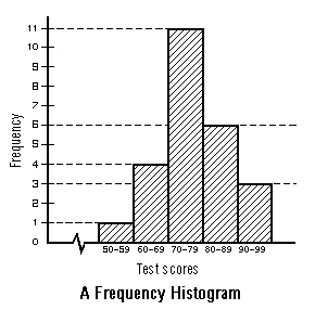
When we deal with large sets of data, a good overall picture and all the information we need can often be conveyed by grouping the data into a number of classes, intervals, or categories. For instance, suppose that a class of 25 students received the following scores on a final exam for a math class,
57, 71, 63, 67, 66, 72, 93, 71, 75, 72, 73, 77, 71, 70, 83, 92, 79, 85, 80, 84, 83, 85, 95, 62, 70, we can summarize them as:

Interval	Tally	Frequency
50 - 59	/	1
60 - 69	////	4
70 - 79	///// ///// /	11
80 - 89	///// /	6
90 - 99	///	3

Frequency distributions present data in a relatively compact form, give a good overall picture, and contain adequate information for many purposes. A quick glance at the table above gives us a good idea of how the test grades are distributed, with most of the scores falling between 70 and 79.

The construction of a frequency distribution consists of three major steps:

Choosing the classes (intervals or categories)

we seldom use fewer than 6 or more than 15 classes
we should make sure that each item goes into one and only one class
whenever possible, we should make the classes cover an equal range of values

Sorting or tallying the data into these classes
Counting the number of items in each class

Frequency Histograms

Histograms are constructed by representing the measurements or observations that are grouped on a horizontal scale and the class frequencies on a vertical scale, and drawing rectangles whose bases equal the class intervals and whose heights are the corresponding class frequencies.

This is the frequency histogram for the final exam scores we obtained previously when we discussed frequency distribution:

Cumulative Frequency Tables

Cumulative frequency tables display, for each given interval, the sum of the number of scores in all preceding intervals up to and including those contained in the interval being studied. It is a way to modify the frequency distribution, making it into a "less than," "or less," "more than," "or more" distribution. To construct a cumulative distribution, we simply add the class frequencies, starting either at the top or at the bottom of the distribution.

Old Interval	Old Frequency	New Interval	Cumulative Frequency
50 - 59	1	50 - 59	1
60 - 69	4	50 - 69	5
70 - 79	11	50 - 79	16
80 - 89	6	50 - 89	22
90 - 99	3	50 - 99	25

Cumulative Frequency Histograms

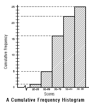
Cumulative frequency histograms are constructed by using the same method as we used for constructing frequency histograms, with the exception that we now add more data to each successive class/interval. In other words, we should be seeing a histogram in which the frequency is increasing.

This is the cumulative frequency histogram for the final exam scores we obtained previously when we discussed frequency distribution:

Range

The range of a set of numbers is the difference between the largest and the smallest numbers of the set. The range of the set 1, 2, 5, 200 is 199, since 200 - 1 = 199. When the range is relatively large, the value of the mean (in this example, 52) may be distorted. This usually reflects the existence of an "outlier".

This is why we need to study measures of dispersion, which indicate whether the data are spread out or are clustered together. Some examples of measures of dispersion include: range, standard deviation, and variance.

Standard Deviation

The standard deviation is the most widely used measure of dispersion. It is defined as the square root of the variance, which is the mean of the squares of the deviation from the mean. In other words, the standard deviation is the measure of how the average deviates from the mean.

Note: Depending on whether the scores you have is from a population or from a sample. The formula for finding standard deviation will change. When the scores are from a sample, instead of dividing the sum of the total deviation by n, you divide that by n-1. The sample standard deviation, s, is equal to:

For example, find the standard deviation of the set (population), 1, 2, 5, 200.
Since the average (mean) of the set is (1 + 2 + 5 + 200) / 4 = 208 / 4 = 52
The sum of the squares of the deviation from the mean is equal to
(200 - 52)^2 + (5 - 52)^2 + (2 - 52)^2 + (1 - 52)^2 = 21904 + 2209 + 2500 + 2601 = 2921
The variance of the set is equal to 29214 / 4 = 7303.5
The standard deviation is equal to 7303.5^(1/2) = 85.5, rounded to the nearest tenth. Since the SD (standard deviation) is considerably bigger than the mean of 52, you can reasonably suspect that the data are widely scattered, rather than clustered around the mean.

Variance

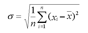
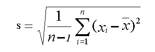
The variance of a set of numbers is the average of the squares of the deviation from the mean. Another way of looking at variance is to think of it as the square of the standard deviation.

Note: If the numbers are from a sample instead of the population, the variance of a sample is equal to:

From the previous example, we know that the standard deviation of the set, 1, 2, 5, 200 is 85.5
The variance of the set is equal to 85.5^2 = 7303.5

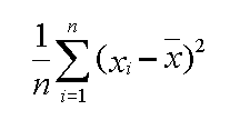
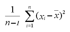
By squaring each deviation from the mean, the variance formula prevents the mean deviation from summing to zero. The squaring process, however, tends to exaggerate the size of the variance in comparison to the values of the individual data items it is describing. The standard deviation (since it is the square root of variance) attempts to correct this weakness of variance.

Normal Curves

Sometimes, the data that you collect might be dispersed in such a way that resemble a bell-shaped curve. We usually call such a curve, the normal curve.

If you know that a set of data is distributed like a normal curve, you can draw conclusions about how far the data are from the mean.

A normal curve is symmetric with respect to the vertical line x = x bar, or the mean. If a set of data values, such as the scores on a test, fits a normal curve, then the numbers of these data values that fall within one, two, and three standard deviations of the mean can be predicted, as shown in the following diagram:

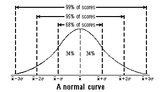
Since 68% of the data values or scores fall within one standard deviation of the mean, and that the curve is symmetric, then it follows that 34% of the data values fall on either side of (one standard deviation from) the mean. Since the normal curve is symmetric about the vertical line x = x bar (the mean), the mean and the median coincide. Hence, 50% of the data values are found on either side of the mean.

When a large number of data points closely approximate the bell shape of a normal curve, the data are said to be approximately normally distributed. When data are normally distributed, the following relationship can be used to draw conclusions concerning the approximate numbers of data scores that are within one, two, and three standard deviations from the mean:

Interval	Interval Length	Contains...
mean +/- one standard deviation	2 standard deviations	68% of all scores
mean +/- two standard deviations	4 standard deviations	95% of all scores
mean +/- three standard deviations	6 standard deviations	99% of all scores

For example, a set of test scores are said to be approximately normally distributed. It has a mean of 75 and a standard deviation of 5. Approximately what percent of the scores fall between 65 and 85? And if 100 students took this test, how many students scored between 65 and 85?

Since one standard deviation is 5, the requested interval is within two standard deviations of the mean. According to the table from above, approximately 95% of the test scores should fall between 65 and 85.

If 100 students took this test, then, 95% of them, or 95 of them would have scored between 65 and 85.

Whether you're considering the validity of a national poll or the virtues of a revolutionary and innovative product, this book will prepare you to make informed judgments on the statistical analyses of others, and, arm you to conduct some random samplings and polls of your own!

Click here to go back to Statistics 101 - Part 1

Do you think you have mastered this topic?

If so, why not take the Statistics Quiz (requires Netscape 3.x or up)?
If you do not have Netscape 3.x or up, then click here for the non-Java version of the Statistics Quiz
Or you can take the Jeopardy Challenge!

[ Home | Regents Review | Join Pen-Pal Network | E-mail me ]