Selected Essays And Book Reviews
COUN 585 - Introduction To Research Methods
WINKS Assignments {4,287 words}
1. Page 2-6, Example 1
WINKS 4.62 January 15,2001
---------------------------------------------------------------------------
Independent Group Analysis C:\WINKS\TTEST.DBF
---------------------------------------------------------------------------
Grouping variable is GROUP
Analysis variable is OBS
Group Means and Standard Deviations
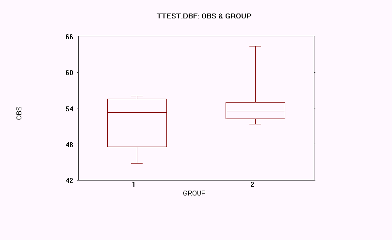
1: mean = 51.4571 s.d. = 4.7476 n = 7
2: mean = 54.9667 s.d. = 4.7944 n = 6
Independent group t-test on OBS
---------------------------------------------------------------------------
Test equality of variance: F = 1.02 with (5, 6) D.F. p = 0.961 (two-tail)
Note: Since the p-value for equality of variance is greater than 0.05,
use the Equal variance t-test results.
Independent Group t-test Hypotheses:
------------------------------------
Ho: There is no difference between means.
Ha: The means are different.
Equal variance: Calculated t= -1.32 with 11 D.F. p = 0.213 (two-tail)
Unequal variance: Calculated t= -1.32 with 10.7 D.F. p = 0.216 (two-tail)
For a one-sided test, you must adjust the p-value according to
the direction of your alternative hypothesis.

2. Page 2-9, Example 2
WINKS 4.62 January 15,2001
---------------------------------------------------------------------------
Descriptive Statistics C:\WINKS\MYDATA.DBF
---------------------------------------------------------------------------
Variable Name is SCORE
N = 15 Missing or Deleted = 0
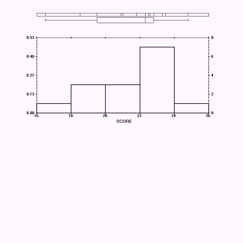
Mean = 21.42 St. Dev (n-1) = 2.26722
Median = 22.30 St. Dev (n) = 2.19034
Minimum = 16.50 S.E.M. = 0.58539
Maximum = 24.80 Variance = 5.14028
Sum = 321.30 Coef. Var. = 0.10585
---------------------------------------------------------------------------
Percentiles: Tukey Five Number Summary:
0.0% = 16.50 Minimum Minimum = 16.50
0.5% = 16.50 25th = 19.50
2.5% = 16.50 Median = 22.30
10.0% = 17.70 75th = 22.80
25.0% = 19.50 Quartile Maximum = 24.80
50.0% = 22.30 Median
75.0% = 22.80 Quartile
90.0% = 24.02
97.5% = 24.80
99.5% = 24.80 Test for normality results:
100.0% = 24.80 Maximum D = .184 p >= 0.20
Five number summary consists of the 0, 25, 50, 75 and 100th percentiles.
Confidence Intervals about the mean:
---------------------------------------------------------------------------
80 % C.I. based on a t(14) critical value of 1.35 is (20.62972, 22.21028)
90 % C.I. based on a t(14) critical value of 1.77 is (20.38385, 22.45615)
95 % C.I. based on a t(14) critical value of 2.15 is (20.1614, 22.6786)
98 % C.I. based on a t(14) critical value of 2.63 is (19.88041, 22.95958)
99 % C.I. based on a t(14) critical value of 2.98 is (19.67553, 23.16447)
The normality test suggests that the data are approx. normally distributed.
The test for normality is a modified Kolmogorov-Smirnov test based on
papers by Lilliefors and Dallal & Wilkinson. References in latenews.txt.
3. Page 4-2, Detailed Statistics and Histograms
Answers to the questions for page 4-2.
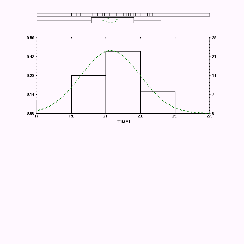
1. The mean = 21.268. The standard deviation = 1.71696 (using the n-1 version). The size of the sample = 50
2. Because p>=0.20, there is evidence to show that the distribution is normal.
3. The raw score at the 90th percentile is 23.50.
4. From looking at the bell curve overlaid on the histogram, the skewness seems to be very minimal. However, it might be slightly skewed to the right (negatively skewed) since the median is greater than the mean.
WINKS 4.62 January 15,2001
---------------------------------------------------------------------------
Descriptive Statistics C:\WINKS\EXAMPLE.DBF
---------------------------------------------------------------------------
Variable Name is TIME1
N = 50 Missing or Deleted = 0
Mean = 21.268 St. Dev (n-1) = 1.71696
Median = 21.30 St. Dev (n) = 1.6997
Minimum = 17.00 S.E.M. = 0.24281
Maximum = 24.20 Variance = 2.94793
Sum = 1063.40 Coef. Var. = 0.08073
---------------------------------------------------------------------------
Percentiles: Tukey Five Number Summary:
0.0% = 17.00 Minimum Minimum = 17.00
0.5% = 17.00 25th = 20.15
2.5% = 17.3025 Median = 21.30
10.0% = 18.91 75th = 22.60
25.0% = 20.15 Quartile Maximum = 24.20
50.0% = 21.30 Median
75.0% = 22.60 Quartile
90.0% = 23.50
97.5% = 24.1175
99.5% = 24.20 Test for normality results:
100.0% = 24.20 Maximum D = .093 p >= 0.20
Five number summary consists of the 0, 25, 50, 75 and 100th percentiles.
Confidence Intervals about the mean:
---------------------------------------------------------------------------
80 % C.I. based on a t(49) critical value of 1.3 is (20.95234, 21.58366)
90 % C.I. based on a t(49) critical value of 1.68 is (20.86007, 21.67593)
95 % C.I. based on a t(49) critical value of 2.01 is (20.77994, 21.75606)
98 % C.I. based on a t(49) critical value of 2.41 is (20.68282, 21.85318)
99 % C.I. based on a t(49) critical value of 2.68 is (20.61726, 21.91874)
The normality test suggests that the data are approx. normally distributed.
The test for normality is a modified Kolmogorov-Smirnov test based on
papers by Lilliefors and Dallal & Wilkinson. References in latenews.txt.
4. Page 4-4 Summary Statistics on a Number of Variables
Answers to the questions for page 4-4.
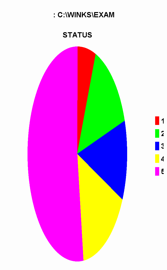
1. Status group 5 has the largest sample size.
2. The potential problem is that the smaller sample size reduces the statistical significance of Status Group 1. Sampling error is inversely proportional to the size of the sample.
WINKS 4.62 January 15,2001
---------------------------------------------------------------------------
Descriptive Statistics, Summary C:\WINKS\EXAMPLE.DBF
---------------------------------------------------------------------------
Statistics from database C:\WINKS\EXAMPLE.DBF Number of records= 50
------ STATUS = 1
FIELD N MEAN STD SEM MIN MAX SUM
----- - ---- --- --- --- --- ---
AGE 3 11.67 1.15 .67 11 13 35
TIME1 3 21.267 1.973 1.139 19 22.60 63.80
------ STATUS = 2
FIELD N MEAN STD SEM MIN MAX SUM
----- - ---- --- --- --- --- ---
AGE 7 9.86 2.48 .94 7 13 69
TIME1 7 21.457 1.420 .537 18.90 23.40 150.20
------ STATUS = 3
FIELD N MEAN STD SEM MIN MAX SUM
----- - ---- --- --- --- --- ---
AGE 6 11.33 2.25 .92 8 13 68
TIME1 6 22.033 1.536 .627 19.30 23.70 132.20
------ STATUS = 4
FIELD N MEAN STD SEM MIN MAX SUM
----- - ---- --- --- --- --- ---
AGE 8 10.50 2.27 .80 6 13 84
TIME1 8 21.538 2.155 .762 18.50 24.20 172.30
------ STATUS = 5
FIELD N MEAN STD SEM MIN MAX SUM
----- - ---- --- --- --- --- ---
AGE 26 10.27 2.65 .52 4 15 267
TIME1 26 20.958 1.714 .336 17 23.90 544.90
5. Page 1-12 Example 2 First Impression Charts
VAR1 VAR2 VAR3 VAR4 VAR5 LABEL
10 20 30 40 50 one
13 14 18 19 18 two
4 29 33 29 10 three
20 21 32 42 21 four
8 9 4 2 9 five
11 4 3 2 3 six
12 12 12 12 12 seven
Answers to the questions for page 1-12.
1. In Group 3, the difference between VAR1 and VAR2 is 25.
2. In Group 7, based on the above data and the below chart shows the least variation between VAR1, VAR2, and VAR3.
![]()
6. Page 4-9 XY Scatterplot
Answers to the questions for page 4-9.
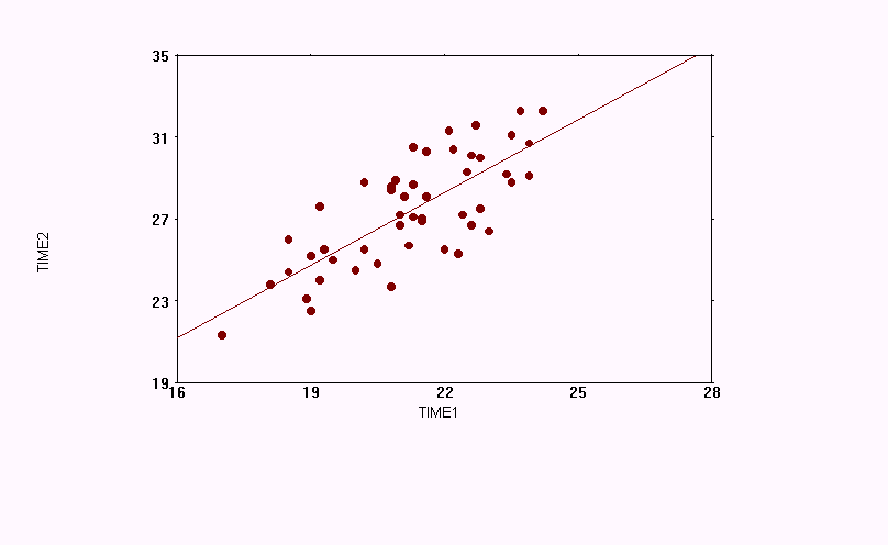
1. The diagram is shown below.
2. TIME1 and TIME2 show a positive correlation to each other based on the positive slope of the line of best fit.
3. With a Correlation Coefficient of 0.764, an R-square of 0.5836, and a Spearman's Coefficient of 0.7361, the relationship between these variables is only moderately strong.
WINKS 4.62 January 15,2001
---------------------------------------------------------------------------
Correlation Coefficients C:\WINKS\EXAMPLE.DBF
---------------------------------------------------------------------------
Variables used : TIME1 and TIME2
Number of cases used: 50
Pearson's r (Correlations Coefficient) = 0.7640 R-Square = 0.5836
Test of hypothesis to determine significance of relationship:
H(null): Slope = 0 or H(null): r = 0
(Pearson's) t = 8.202562 with 48 d.f. p < 0.001
(A low p-value implies that the slope does not = 0.)
Spearman's Rank Correlation Coefficient = 0.7361
(Spearman's) t = 7.535245 with 48 d.f. p < 0.001
7. Page 4-9 & I-8 Histogram/Stats
Answers to the questions for page 4-9 & I-8.
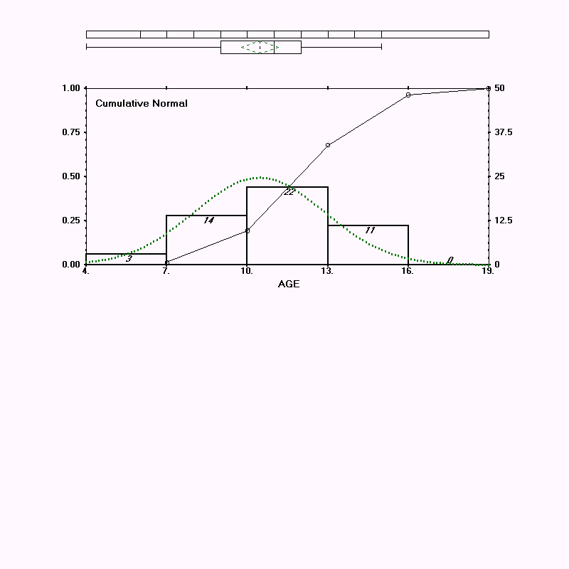
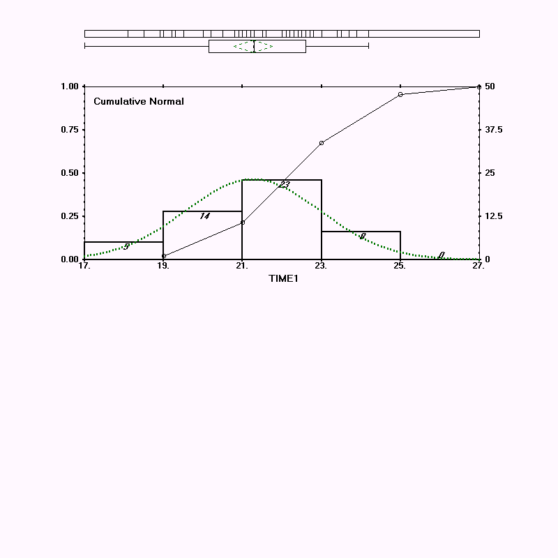
1. On AGE, as shown below, the distribution will be normal if there are 3 fewer 4-6 year olds and 3 fewer 7-10 year olds. On TIME1, the curve would be more normal if the researcher had 5 fewer times between 19 and 21, and 5 more times between 25 and 27.
8. Page 4-11 Displaying By-group Plots
Answers to the questions for page 4-11.
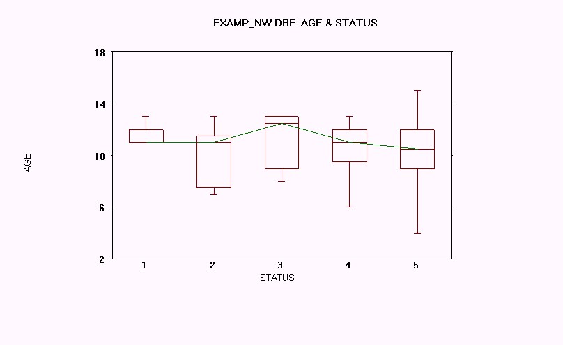
1. Because of the wide range of values in Group 5, I would say that that group has outliers.
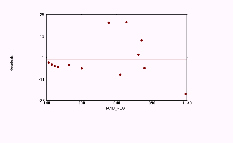
2. Outliers are points that are significantly outside a smooth least squares fit. They can be identified by their large residuals.
3. The line of connected medians sort of looks like a Normal distribution.
4. The horizontal line through each box represents the median for each status.
9. Page 4-18 Two-Sample t-Test (Independent Groups)
Answers to the questions for page 4-18.
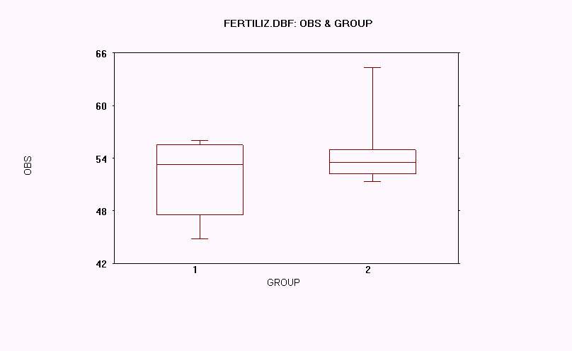
1. The p-value for this test is p = 0.961. Since it is greater than 0.5, the variances are considered equal, and the test is significant.
2. We would use the Equal variance t-test.
3. For the Equal variance t-test, t= -1.32 with 11 degrees of freedom, and p = 0.213 (two-tail)
4. With p=0.213 and much greater than the significance level of 0.05, the null hypothesis of "no difference between means" is not rejected.
WINKS 4.62 January 16,2001
---------------------------------------------------------------------------
Independent Group Analysis C:\WINKS\FERTILIZ.DBF
---------------------------------------------------------------------------
Grouping variable is GROUP
Analysis variable is OBS
Group Means and Standard Deviations
1: mean = 51.4571 s.d. = 4.7476 n = 7
2: mean = 54.9667 s.d. = 4.7944 n = 6
Independent group t-test on OBS
---------------------------------------------------------------------------
Test equality of variance: F = 1.02 with (5, 6) D.F. p = 0.961 (two-tail)
Note: Since the p-value for equality of variance is greater than 0.05,
use the Equal variance t-test results.
Independent Group t-test Hypotheses:
------------------------------------
Ho: There is no difference between means.
Ha: The means are different.
Equal variance: Calculated t= -1.32 with 11 D.F. p = 0.213 (two-tail)
Unequal variance: Calculated t= -1.32 with 10.7 D.F. p = 0.216 (two-tail)
For a one-sided test, you must adjust the p-value according to
the direction of your alternative hypothesis.
10. Page 4-21 One-Way Anova Example
Answers to the questions for page 4-21.
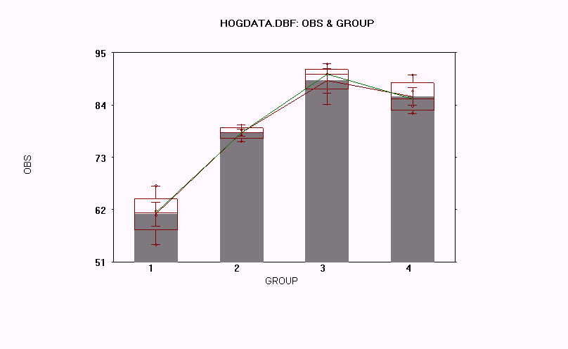
1. Because of the low p-value (p<.001), the test for an equality of variance shows that there is a difference between groups and that the difference is not due to chance.
2. A larger sample would be good, but using Degrees of Freedom means that the test can still be valid. The sample is also well distributed across the 4 groups.
3. The t-Test is performed when there are 2 groups, and an ANOVA is performed when there are 3 to 10 groups.
4. Means 3 and 4 did not differ significantly.
5. Group 2 means had the least amount of variability.
6. Groups 3 and 4 had means that were significantly greater than the other two.
WINKS 4.62 January 16,2001
---------------------------------------------------------------------------
Independent Group Analysis C:\WINKS\HOGDATA.DBF
---------------------------------------------------------------------------
Grouping variable is GROUP
Analysis variable is OBS
Group Means and Standard Deviations
1: mean = 61.025 s.d. = 5.0822 n = 4
2: mean = 78.125 s.d. = 1.4886 n = 4
3: mean = 89.0667 s.d. = 4.4276 n = 3
4: mean = 85.775 s.d. = 3.5976 n = 4
Analysis of Variance Table
Source S.S. DF MS F Appx P
---------------------------------------------------------------------------
Total 1923.41 14
Treatment 1761.24 3 587.08 39.82 <.001
Error 162.17 11 14.74
Error term used for comparisons = 14.74 with 11 d.f.
Critical q
Newman-Keuls Multiple Comp. Difference P Q (.05)
-----------------------------------------------------------------------------------------
Mean(3)-Mean(1) = 28.0417 4 13.523 4.256 *
Mean(3)-Mean(2) = 10.9417 3 5.277 3.82 *
Mean(3)-Mean(4) = 3.2917 2 1.587 3.113
Mean(4)-Mean(1) = 24.75 3 12.892 3.82 *
Mean(4)-Mean(2) = 7.65 2 3.985 3.113 *
Mean(2)-Mean(1) = 17.1 2 8.907 3.113 *
Homogeneous Populations, groups ranked
Gp Gp Gp Gp
1 2 4 3
------
---
---
This is a graphical representation of the Newman-Keuls multiple comparisons
test. At the 0.05 significance level, the means of any two groups
underscored by the same line are not significantly different.
11. Page 4-25 Paired t-Test Repeated Measures
Answers to the questions for page 4-25.
1. The repeated measures test is used when observations are to be taken on the same or similar subjects over time, and the before and after results are not independent of each other.
2. With p=.0076, there is evidence to reject the null hypothesis and assume that there is a difference between the before and after weights of the subjects.
3. A Type-1 error is that the researcher would reject the null hypothesis when it is true. By choosing a significance level of 0.05, this is saying that there are 5 chances out of 100 that the null hypothesis will be rejected when it is true.
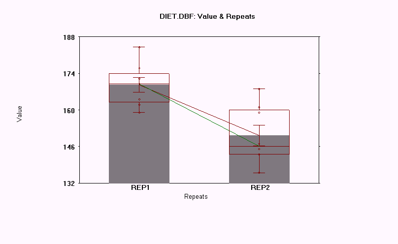
4. The subjects mean scores did differ significantly over time. Their average weight before was 169.625, and after, it was 150.25.
WINKS 4.62 January 16,2001
---------------------------------------------------------------------------
Repeated Measures Analysis Summary C:\WINKS\DIET.DBF
---------------------------------------------------------------------------
Number of repeated measures is 2
Number of subjects read in 8
Means and standard deviations for 2 repeated measures:
1)REP1: mean = 169.625 s.d. = 8.07001
2)REP2: mean = 150.25 s.d. = 11.04213
Mean Difference = 19.375 s.d.(difference) = 14.78356
95% C.I. about Mean Difference is (7.01367, 31.73633)
Paired t-test
--------------
Hypotheses:
Ho: The mean difference between pairs is 0.
Ha: The mean difference between pairs is not 0.
Calculated t = 3.70687 with 7 D.F. p = 0.0076 (two-sided)
Since p <= 0.05, at the 0.05 significance level you have evidence
to reject the null hypothesis and conclude that the mean difference
between pairs is not 0.
For a one-sided test, you must adjust the p-value according to
the direction of your alternative hypothesis.
12. Page 4-28 Example One-Way Repeated Measures ANOVA
Answers to the questions for page 4-28.
1. There are more than a pair of repeated measures in this test because subjects will be taking four different drugs. Also, the test on page 4-25 involved dependent variables, and this one involves independent variables.
2. There are 4 independent variables because none of the variables get their value based on another variable.
3. There are 5 levels of independent variables in this analysis.
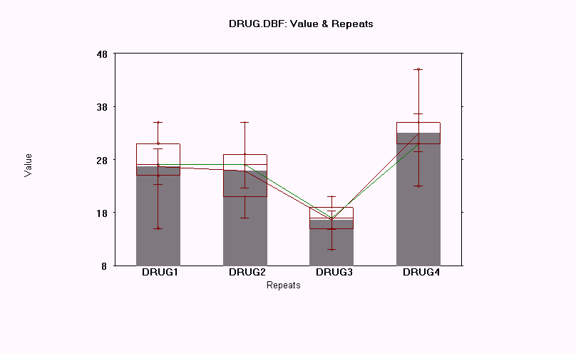
4. The value of "F" is 29.99, and the value of "p" is less than 0.001. The low p-value means that there is a significant difference in the mean response times of the 4 drugs.
5. The means of Groups 1 and 2 are not significantly different.
6. Drug 4 produced the largest mean response. The difference was significantly larger than the other 3, but it was especially larger than Drug 3.
WINKS 4.62 January 16,2001
---------------------------------------------------------------------------
Repeated Measures Analysis Summary C:\WINKS\DRUG.DBF
---------------------------------------------------------------------------
Number of repeated measures is 4
Number of subjects read in 5
Means and standard deviations for 4 repeated measures:
1)DRUG1: mean = 26.6 s.d. = 7.53658
2)DRUG2: mean = 25.8 s.d. = 7.01427
3)DRUG3: mean = 16.6 s.d. = 3.84708
4)DRUG4: mean = 33.0 s.d. = 8.0
Repeated Measures Analysis of Variance
Source -----S.S.----- --DF-- MS F Appx p
---------------------------------------------------------------------------
Between Subject 648.00 4
Within Subject 775.00 15
Rep. Factor 683.80 3 227.93 29.99 <.001
Error 91.2 12 7.60
---------------------------------------------------------------------------
Total 1423.00 19
Error term used for comparisons = 7.6 with 12 d.f.
Critical q
Newman-Keuls Multiple Comp. Difference P Q (.05)
------------------------------------------------------------------------
Mean( 4)-Mean( 3) = 16.4 4 13.302 4.199 *
Mean( 4)-Mean( 2) = 7.2 3 5.84 3.773 *
Mean( 4)-Mean( 1) = 6.4 2 5.191 3.082 *
Mean( 1)-Mean( 3) = 10.0 3 8.111 3.773 *
Mean( 1)-Mean( 2) = 0.8 2 .649 3.082
Mean( 2)-Mean( 3) = 9.2 2 7.462 3.082 *
Homogeneous Populations, repeated measures ranked
Gp 1 refers to DRUG1
Gp 2 refers to DRUG2
Gp 3 refers to DRUG3
Gp 4 refers to DRUG4
Gp Gp Gp Gp
3 2 1 4
------
---
---
This is a graphical representation of the Newman-Keuls multiple comparisons
test. At the 0.05 significance level, the means of any two groups
underscored by the same line are not significantly different.
13. Page 4-43 Simple Linear Regression
Answers to the questions for page 4-43.
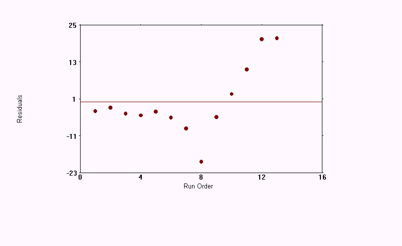
1. The dependent variable was Homicide Rate, and the independent variable was Handguns Registered.
2. The intercept tells the number of homicides when there are no handguns registered. In this example, it is 4.910512.
3. The magnitude is 0.03761144 and is positive.
4. The correlation coefficient, 0.7263, shows neither strength or weakness in the correlation. A low p-value of 0.005 suggests that the dependent variable HOM_RATE may be linearly related to independent variable(s).
5. The probability that the slope=0 (no correlation) is 0.005.
6. Ideally, the sum of the residuals should be zero. That is why least squares uses the squares of the differences.
7. Based on r=.7263, 52.8% of the variance in the dependent variable is because of the independent variable.
8. As handgun registration decreases, homicide rates DECREASE.
WINKS 4.62 January 16,2001
---------------------------------------------------------------------------
Linear Regression and Correlation C:\WINKS\HANDGUNS.DBF
---------------------------------------------------------------------------
Dependent variable is HOM_RATE, 1 independent variables, 13 cases.
---------------------------------------------------------------------------
Variable Coefficient St. Error t-value p(2 tail)
---------------------------------------------------------------------------
Intercept 4.9105126 6.6274622 .7409341 0.474
HAND_REG .0376114 .0107324 3.5044807 0.005
---------------------------------------------------------------------------
R-Square = 0.5275 Adjusted R-Square = 0.4846
Analysis of Variance to Test Regression Relation
Source Sum of Sqs df Mean Sq F p-value
---------------------------------------------------------------------------
Regression 1699.557 1 1699.557 12.281385 0.005
Error 1522.2328 11 138.3848
---------------------------------------------------------------------------
Total 3221.7897 12
A low p-value suggests that the dependent variable HOM_RATE
may be linearly related to independent variable(s).
---------------------------------------------------------------------------
MEAN X = 537.507 S.D. X = 316.415 CORR XSS = 1201423.0
MEAN Y = 25.127 S.D. Y = 16.385 CORR YSS = 3221.788
REGRESSION MS= 1699.557 RESIDUAL MS= 138.385
---------------------------------------------------------------------------
Pearson's r (Correlation Coefficient)= 0.7263
The linear regression equation is:
HOM_RATE = 4.910512 + 3.761144E-02 * HAND_REG
Test of hypothesis to determine significance of relationship:
H(null): Slope = 0 or H(null): r = 0 (two-tailed test)
t = 3.5 with 11 degrees of freedom p = 0.005
Note: A low p-value implies that the slope does not = 0.

14. Page 4-47 Example Multiple Linear Regression Analysis
Answers to the questions for page 4-47.
1. A low p-value for the given coefficient suggests a relationship between the dependent and independent variable. The independent variables that have significant predictive power are UNEMP (p=0.003), ARMED (p<0.001), and TIME (p=0.003).
2. With an R-square=0.9555 and an adjusted R-square=0.9925, the Regression equation is a good fit. The p-value for the Regression equation is less than 0.001, and this is also very good.
3. TIME (with R-square=0.9435 and p<0.001) is the most predictive independent variable. In separate simple linear regression analyses, UNEMP had an R-square of 0.2525 (p=0.047), and ARMED had an R-square of 0.2091 (p=0.075).
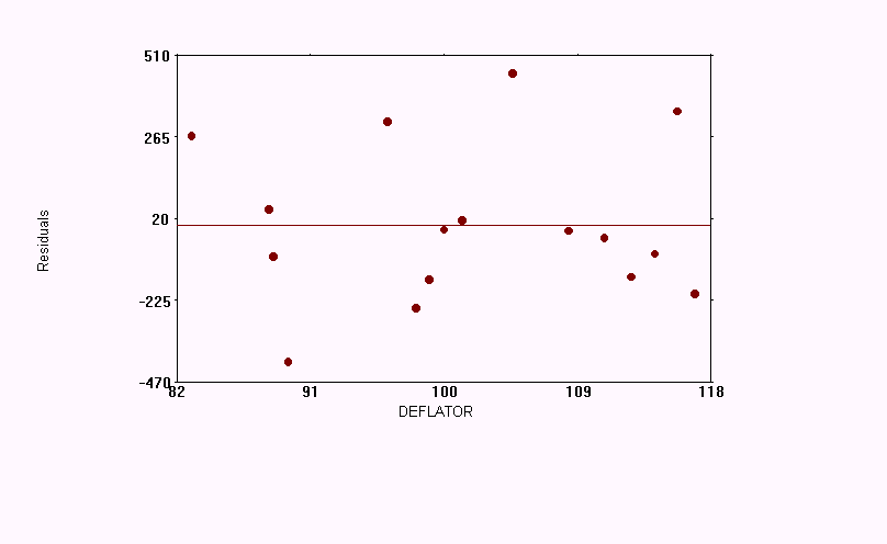
4. As the size of the residuals increase, the error of measurement should also increase.
WINKS 4.62 January 17,2001
---------------------------------------------------------------------------
Linear Regression and Correlation C:\WINKS\LONGLEY.DBF
---------------------------------------------------------------------------
Dependent variable is TOTAL, 6 independent variables, 16 cases.
---------------------------------------------------------------------------
Variable Coefficient St. Error t-value p(2 tail)
---------------------------------------------------------------------------
Intercept -3482258.6349 889652.92 -3.914177 0.004
DEFLATOR 15.061872 84.841736 .177529 0.863
GNP -.0358192 .0334621 -1.070439 0.312
UNEMP -2.02023 .4879787 -4.139996 0.003
ARMED -1.033227 .2140895 -4.826145 <.001
POP -.0511041 .2258783 -.2262461 0.826
TIME 1829.1515 455.08592 4.0193541 0.003
---------------------------------------------------------------------------
R-Square = 0.9955 Adjusted R-Square = 0.9925
Analysis of Variance to Test Regression Relation
Source Sum of Sqs df Mean Sq F p-value
---------------------------------------------------------------------------
Regression 184173843.173 6 30695640.5288 330.85802 <.001
Error 834982.83 9 92775.87
---------------------------------------------------------------------------
Total 185008826. 15
A low p-value suggests that the dependent variable TOTAL
may be linearly related to independent variable(s).
15. Page 4-50 Example Calculating Correlation Coefficients
Answers to the questions for page 4-50.
1. In the previous case, HOM_RATE was assumed to be dependent on HAND_REG. In this case, both variables are assumed to be independent of the other.
2. The null hypothesis, r=0, tests whether or not the two variables have a linear relationship to each other.
3. In the top right chart, HOM_RATE is the dependent variable (y-axis), and HAND-REG is the independent variable (x-axis). In the lower left chart, the two variables and their roles as dependent and independent are reversed.
4. In example 4-43, HOM_RATE was the dependent variable and never considered as the independent variable.
WINKS 4.62 January 17,2001
---------------------------------------------------------------------------
Correlation Coefficients C:\WINKS\HANDGUNS.DBF
---------------------------------------------------------------------------
Variables used : HOM_RATE and HAND_REG
Number of cases used: 13
Pearson's r (Correlations Coefficient) = 0.7263 R-Square = 0.5275
Test of hypothesis to determine significance of relationship:
H(null): Slope = 0 or H(null): r = 0
(Pearson's) t = 3.504481 with 11 d.f. p = 0.005
(A low p-value implies that the slope does not = 0.)
Spearman's Rank Correlation Coefficient = 0.7527
16. Page 4-52 & 4-53 Example Graphical Correlation Matrix
Answers to the questions for page 4-52 & 4-53.
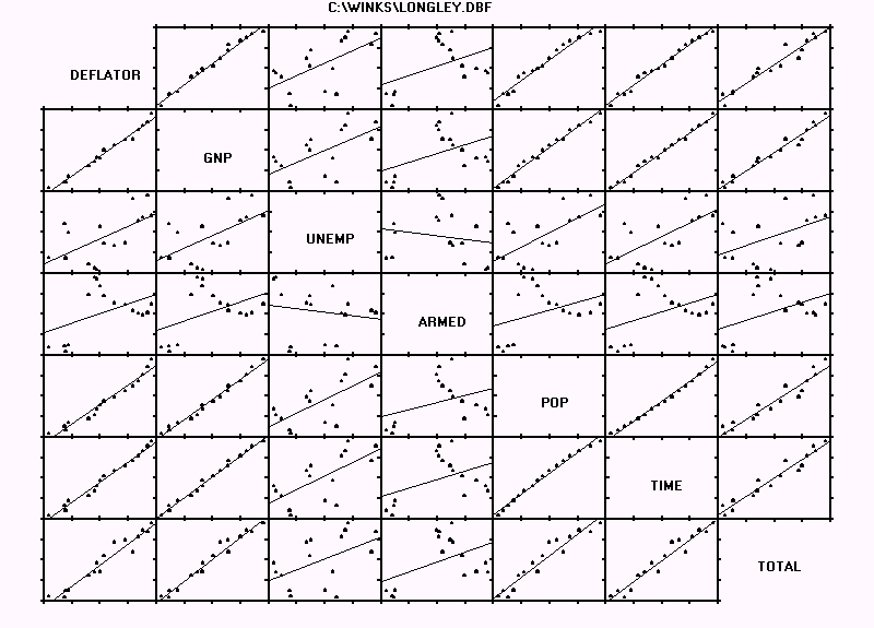
1. UNEMP and ARMED have the weakest correlation (r=-0.177 and p=.511) based on magnitude of "r", not the sign. GNP and TIME have the strongest simple correlation based on r=0.995 and p=0.0.
2. ARMED appears to have large residual values when correlated with all the other variables because it seems to have a non-linear relationship to most of them.
WINKS 4.62 January 17,2001
---------------------------------------------------------------------------
Matrix of Correlation Coefficients C:\WINKS\LONGLEY.DBF
---------------------------------------------------------------------------
DEFLAT GNP UNEMP ARMED POP TIME TOTAL
DEFLATOR .992 .621 .465 .979 .991 .971
( 0.0) (0.01) (0.07) ( 0.0) ( 0.0) ( 0.0)
[ 16] [ 16] [ 16] [ 16] [ 16] [ 16]
GNP .604 .446 .991 .995 .984
(.013) (.083) ( 0.0) ( 0.0) ( 0.0)
[ 16] [ 16] [ 16] [ 16] [ 16]
UNEMP -.177 .687 .668 .502
(.511) (.003) (.005) (.047)
[ 16] [ 16] [ 16] [ 16]
ARMED .364 .417 .457
(.165) (.108) (.075)
[ 16] [ 16] [ 16]
POP .994 .96
( 0.0) ( 0.0)
[ 16] [ 16]
TIME .971
( 0.0)
[ 16]
TOTAL
-------------------------------------------------------------------------------------------------------
Key: Correlation
(p-value)
[count]
17. Page 4-55 Frequencies Analysis
Answers to the questions for page 4-55.
1. Because the EXAMPLE database is dealing with categorical type data, the Chi-square test would be the tool that would best compliment the evaluation of frequencies in this example. The regression tools test relationships between variables, and the t-Test and ANOVA tools test variances to determine if differences between variables are significant.
2. I prefer the bar chart because it is easier to see if one frequency is significantly different than the others. Because of the y-axis labeling, it is also easier to know the exact frequencies of the statuses.
WINKS 4.62 January 17,2001
---------------------------------------------------------------------------
Frequency Tables C:\WINKS\EXAMPLE.DBF
---------------------------------------------------------------------------
Number of records in database = 50
Frequency Table for STATUS
Cumulative Cumulative
STATUS Frequency Percent Frequency Percent
-----------------------------------------------------------
1 3 6.0 3 6.0
2 7 14.0 10 20.0
3 6 12.0 16 32.0
4 8 16.0 24 48.0
5 26 52.0 50 100.0
![]()
![]()
18. Page 5-2 Two-Way ANOVA
Answers to the questions for page 5-2.
1. HEIGHT and WIDTH are the two independent variables in this example.
2. There are 3 levels of each independent variable.
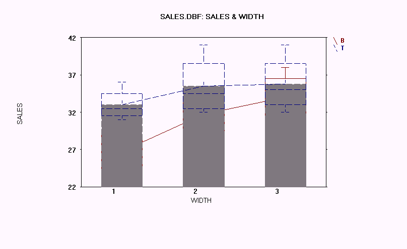
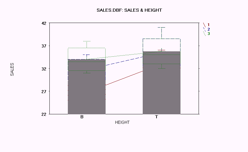
3. The p-value for INTERACTION is 0.395, and this is well above 0.05. Therefore, the interaction effect cannot be considered significant. Failure for the means of the variables to intersect in the interaction plots also indicates that no interaction effect exists.
4. When no interaction effect exists, the next appropriate action is to look at the means of HEIGHT and WIDTH.
5. The p-value for HEIGHT is 0.008 and for WIDTH is 0.016. Both of these values are well below 0.05, so this means that each variable was significant in accounting for the number of SALES.
6. HEIGHT has the two levels of TOP and BOTTOM, and TOP was the choice that yielded the greater sales. For WIDTH, there are three levels, and WIDTH2 and WIDTH3, over WIDTH1, both led to about the same number of sales.
7. The failure of the means of the variables to intersect (and to be close to parallel) are evidence that no interaction effect occurred.
WINKS 4.62 January 18,2001
---------------------------------------------------------------------------
Two-Way Analysis of Variance C:\WINKS\SALES.DBF
---------------------------------------------------------------------------
Data Summary:Cell means, standard deviation and counts...
HEIGHT |B |T
---------------------
WIDTH | 26.75 | 33.0|
| 2.75 | 2.16|
|1 n = 4| n = 4|
---------------------
| 31.75| 35.5|
| 2.99| 4.04|
2| n = 4| n = 4|
---------------------
| 34.0| 35.75|
| 3.16| 3.86|
3| n = 4| n = 4|
---------------------
HEIGHT is a Fixed Factor. WIDTH is a Fixed Factor.
Analysis of Variance Table
Source S.S. DF MS F P
---------------------------------------------------------------------------
Total 407.96 23
Cells 220.71 5
WIDTH 108.33 2 54.17 5.21 0.016
HEIGHT 92.04 1 92.04 8.85 0.008
INTERACTION 20.33 2 10.17 .98 0.395
Within Cells 187.25 18 10.40
---------------------------------------------------------------------------
If the interaction effect is considered non-significant,
multiple comparisons of marginal means is appropriate.
The following multiple comparisons will be performed:
Marginal means comparisons:
MAIN EFFECTS (Compare marginal means) - HEIGHT Number of levels = 2
HEIGHT (Marginal means)
Means compared are:
HEIGHT(Gp) 1 = B) Mean= 30.83333 n = 12
HEIGHT(Gp) 2 = T) Mean= 34.75 n = 12
Error term used for comparisons = 10.4 with 18 d.f.
Critical q
Newman-Keuls Multiple Comp. Difference P Q (.05)
------------------------------------------------------------------------
Mean(T)-Mean(B) = 3.9167 2 4.207 2.971 *
Homogeneous Populations, groups ranked
Gp Gp
B T
---
---
This is a graphical representation of the Newman-Keuls multiple comparisons
test. At the 0.05 significance level, the means of any two groups
underscored by the same line are not significantly different.
MAIN EFFECTS (Compare marginal means) - WIDTH Number of levels = 3
WIDTH (Marginal means)
Means compared are:
WIDTH(Gp) 1 = 1) Mean= 29.875 n = 8
WIDTH(Gp) 2 = 2) Mean= 33.625 n = 8
WIDTH(Gp) 3 = 3) Mean= 34.875 n = 8
Error term used for comparisons = 10.4 with 18 d.f.
Critical q
Newman-Keuls Multiple Comp. Difference P Q (.05)
------------------------------------------------------------------------
Mean(3)-Mean(1) = 5.0 3 4.385 3.609 *
Mean(3)-Mean(2) = 1.25 2 1.096 2.971
Mean(2)-Mean(1) = 3.75 2 3.289 2.971 *
Homogeneous Populations, groups ranked
Gp Gp Gp
1 2 3
------
---
This is a graphical representation of the Newman-Keuls multiple comparisons
test. At the 0.05 significance level, the means of any two groups
underscored by the same line are not significantly different.
Tom of Bethany
"He that hath the Son hath life; and he that hath not the Son of God hath not life." (I John 5:12)
"And ye shall seek me, and find me, when ye shall search for me with all your heart." (Jeremiah 29:13)
Index to Selected Essays And Book Reviews
GLA 2. Violent Media Alone Does Not Produce Children With Aggressive Behavior
Send email to:
tlee6040@aol.com