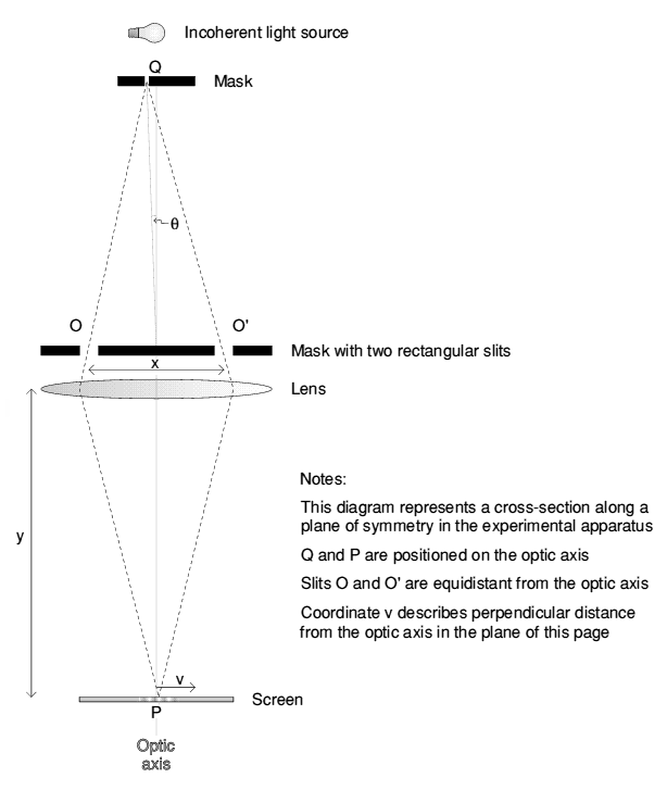
The American physicist A. A. Michelson demonstrated the practicability of measuring light sources using optical interferometry² in 1890 with the experimental apparatus shown in Figure 1.

Figure 1 - Michelson?s experimental apparatus

Various masks were placed in front of incoherent light sources, acting as "artificial stars" for the experiment. Light from a distant artificial star passed through slits O and O' and was then focused by a lens of focal length y to form an image on the screen. In a mathematical analysis of this experiment it is easier to first consider a monochromatic point source at Q on the optic axis. Spherical wavefronts will radiate from the source reaching slits O and O' simultaneously. Light passing through slit O will interfere with light passing through slit O' forming intensity fringes on the screen either side of point P. The optical path length from Q to point P on the screen is the same for rays travelling through either slit. This will not be the general case for light rays travelling to an arbitrary point on the screen from Q. The difference in optical path length between light rays travelling via slit O and those travelling via O' will then be to a first approximation, where v is the co-ordinate on the screen shown in Figure 1. When light rays from the two slits are combined on the screen they will interfere producing intensity proportional to , where k is the wavenumber defined as . Light rays from a point source offset from Q by an angle as shown in Figure 1 give light intensity on the screen proportional to . An extended incoherent source placed at Q can be considered as a distribution of many such point sources. A chromatic source can be considered as the superposition of many monochromatic sources of different frequency. The intensity observed on the screen will be the sum of the intensities produced by each point on the source.

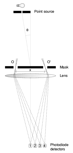
Michelson was not able to make quantitative measurements of the visibility of interference fringes on the screen but did make measurements of the slit separation x which gave minimum fringe visibility. The size of the artificial star can be calculated from this measurement provided its shape and distance are known. With modern photodiode detectors it is possible to make accurate intensity measurements and hence calculate fringe visibilities. The viewing screen is replaced by four light intensity detectors as shown in Figure 2. Detector 1 is positioned so that the optical path lengths from the detector to slit O and from the detector to slit O' are equal. Detector 2 is positioned so that the optical path lengths to O and O' differ by a ¹/₄ of the mean wavelength. For detectors 3 and 4 the path differences are ¹/₂ of a wavelength and ³/₄ of a wavelength respectively. If A is the complex amplitude of the light arriving at detector 1 along the path through slit O, the amplitude of the light arriving via slit O' will be Aexp[-i kx], giving a total amplitude of A+Aexp[-i kx]. The intensity at detector 1 will be:

Similarly if A is the amplitude of the light arriving at detector 2 along the path through slit O, the intensity at the detector will be:

For detector 3:

For detector 4:

I have defined the complex fringe intensity I as (I₁-I₃)+i(I₂-I₄) where I₁ to I₄ are the intensities shown above, and i is . In the case of the point source shown in Figure 2

Figure 2 - Visibility measurement	Figure 3 - Alternative optical arrangement

As the complex intensity I is a linear combination of intensities, the complex intensity of an extended incoherent source can be calculated by summing the contributions from each point on the source. The amplitude A( ) of the light received from points between and +d on the source will be dependent on the source brightness distribution B ( ) in the following manner:

The complex intensity for light received between and +d will be I( )=4B( )exp[i kx] d . Integrating over all gives:

If the variable u is defined as u=kx, then I_TOTAL is proportional to the Fourier transform of the one dimensional source brightness distribution B( ) with respect to u. If this Fourier transform is normalised to have a total intensity of unity we obtain the complex visibility:

Michelson did not have sensitive electronic detectors so his measurements relied on human eyesight. He succeeded in calculating the diameters of Jupiter's satellites ³ using an aperture mask with two slits of adjustable separation placed over the objective of a 12-inch telescope. He measured the slit separations at which the fringes were least visible, and calculated the diameters of the satellites by assuming them to be circular disks with uniform illumination. His results agreed well with visual estimations of the satellite diameters which had been made using large optical telescopes.

With the optical arrangement of Figure 2 a large objective lens or mirror is required for measurements with large slit separations and much of the light that passes through the slits in the aperture mask is wasted. Figure 3 shows an alternative optical arrangement which uses separate optical elements for the two beams. The incident light is from a distant point source at angle . Light entering each of the slits is split into four equal beams which are then directed to the detectors. The path differences between rays travelling through O and O' to each of the detectors are the same as in Figure 2, but in this arrangement all the light entering the apparatus is used efficiently. In practice glass blocks might produce reflections within the apparatus and would probably not be used. Instead, the appropriate difference in optical path length from the detectors to each of the slits could be produced by careful adjustment of the mirror positions. By varying the optical path length of one of the beams it is possible to calculate the complex visibility with just one detector. As the optical path length is varied the interference fringes will be scanned past the detector. The amplitude and phase of the intensity variations at the detector will be linearly related to the amplitude and phase of the complex visibility. In most modern interferometers the intensity variation with time is Fourier transformed to give an amplitude and phase for the complex visibility.

In 1891 Michelson ⁴ discussed the possibility of obtaining information about the brightness distribution within a source from interferometric measurements. He conceded that this was not practicable as it would require accurate measurements of fringe visibility at many different slit separations. Over the next sixty years most of the work on optical interferometry concentrated instead on the measurement of stellar diameters and the separation of binary stars⁵. In 1920 A. A. Michelson and F. G. Pease⁶ constructed a separate-element Michelson stellar interferometer as shown in Figure 4. The separation of the siderostat mirrors was equivalent to the slit separation in his earlier interferometers. Separations of over 20ft were possible, enabling measurements of the diameters of several large stars to be performed. An interferometer with a 50ft siderostat separation ⁷ was built in 1930, with mirrors attached to 9 tons of steel girderwork on the front of a 40 inch optical telescope. Very few astronomical measurements were made with this instrument due to the difficulty of operating it. With both of these interferometers atmospheric fluctuations produced phase variations which caused the fringes to "shimmer", making observation extremely difficult. R. Hanbury Brown⁸ estimated that atmospheric fluctuations may have led to errors of between ten and twenty percent in Michelson and Pease's stellar diameter calculations. Hanbury Brown produced more accurate measurements using an intensity interferometer in Navarra ⁸. Intensity interferometers look at the statistical relationship between the intensities at two separated detectors observing a distant source. Quantum mechanics suggests that this is related to the amplitude of the complex visibility function, allowing measurements of visibility with large detector separations. Unfortunately the phase of the complex visibility cannot be determined, and accurate visibility amplitudes can only be calculated for bright astronomical sources.

Figure 4 - Simple separate element interferometer

Return to Bob's Home Page.