% pipe.m
	%  
	%%%%%%%%%%%%%%%%%%%%%%%%%%%%%%%%%%%%%%%%%%%%
	%          build the chain matrix          %
	%    a pipe of a lossless pipe length l    %
	%                                          % 
	%            Paul Darlington               %
	%                                          %
	%          Paul@appledynamics.com          %
	%                                          %
	%%%%%%%%%%%%%%%%%%%%%%%%%%%%%%%%%%%%%%%%%%%%
	%
	% Input variables......
	% length=l
	% cross sectional area s
	% vector of frequencies = freq

	function [chain] = pipe(l,s,freq)

	omega=2*pi*freq;
	c=340;
	kL=(l/c)*omega;
	rhocs=415/s;

	% Build chain matrix

	chain(1,1,:)=cos(kL);
	chain(1,2,:)=j*rhocs*sin(kL);
	chain(2,1,:)=j/rhocs*sin(kL);
	chain(2,2,:)=cos(kL);
	

This code returns a complex 2*2*n matrix, where n is the number of points in the frequency vector.

Return to the main "two port" page

	% lschain.m
	% 
	%%%%%%%%%%%%%%%%%%%%%%%%%%%%%%%%%%%%%%%%%%%%
	%     build a loudspeaker chain matrix     %
	%                                          %
	%            Paul Darlington               %
	%                                          %
	%          Paul@appledynamics.com          %
	%                                          %
	%%%%%%%%%%%%%%%%%%%%%%%%%%%%%%%%%%%%%%%%%%%%
	%
	% 	Input variables....
	%	s 	cone area
	%	bl 	motor constant
	%	zeb 	electrical blocked impedance	(vector of n elements)
	%	zm 	mechanical impedance 		(vector of n elements)
	%	freq	Frequencies			(vector of n elements)
	
	function [chain] = lschain(s,bl,eb,zm,f)
	
	omega=2*pi*f;
	chain(1,1,:)=s*zeb/bl;
	chain(1,2,:)=(zeb.*zm+bl^2*cos(0*omega))/bl;
	chain(2,1,:)=(s/bl)*cos(0*omega);
	chain(2,2,:)=(1/bl)*zm;
	

This code returns a complex 2*2*n matrix, where n is the number of points in the frequency vector.

Return to the main "two port" page

	% piston.m
	% 
	%%%%%%%%%%%%%%%%%%%%%%%%%%%%%%%%%%%%%%%%%%%%
	%     approximate piston functions         %
	%using series expansions in Kinsler & Frey %
	%            Paul Darlington               %
	%                                          %
	%          Paul@appledynamics.com          %
	%                                          %
	%%%%%%%%%%%%%%%%%%%%%%%%%%%%%%%%%%%%%%%%%%%%
	%
	% 	Input variables....
	%	input 	vector of 2ka's
	
	function y=piston(input)

	r1=input.^2/8;
	x1=input/3;
	N=64;
	blanking=input./input;

	for counter=1:length(input)
	   if input(counter)<30,blanking(counter)=0;end
	end
	overinput=input.*blanking;
	underinput=input.*(1-blanking);
	blanking;
	for j=2:N
	   numer=2;
	   numei=1;
	   for k=2:j   
	      numer=numer*(2*k)^2;
	   end
	   for k=2:j
	      numei=numei*(2*k-1)^2;
	   end
	   numer=numer*2*(j+1);
	   numei=numei*(2*j+1);
	   r1=r1+(-1)^(j-1)*underinput.^(2*j)/numer;   
	   x1=x1+(-1)^(j-1)*underinput.^(2*j-1)/numei;
	end 
	
	r1=r1.*(1-blanking)+blanking;
	imaginover=1./input;
	x1=x1.*(1-blanking)+blanking.*imaginover;
	   
	y=r1+i*4*x1./pi;

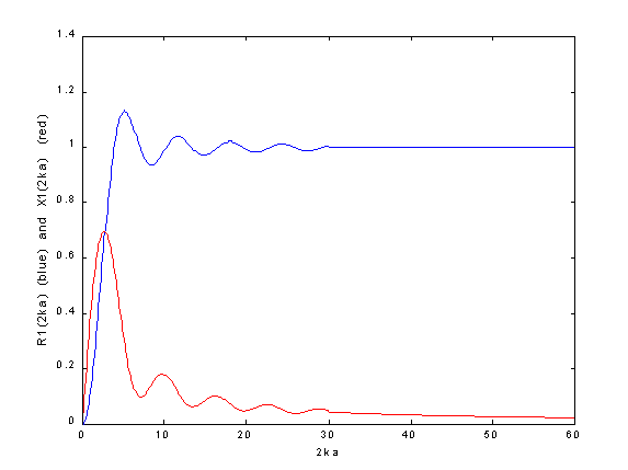
The routine uses a series which is convergent up to input values of 30 - above this a simplified expression is used.

An example of the output from piston.m is shown below:

Compare this with Figure 7.10 of Kinsler & Frey ( First edition).

Do yourself a favour - try to find a first edition of Kinsler & Frey - if not, a second edition is OK. Shame about the third edition !

Return to the main "two port" page