
ELASTICITY
ELASTICITY: response, or D, one variable as a result from the D another variable
Most common measure of elasticity Ä
PRICE ELASTICITY OF
DEMAND
how
much will Qd D, when there is a D
Price ??????
a measure of the % D
Qd
divided by the % D
P
% DQd DQd
Ed =
= Qd
DP
% DP
P
* Use the same formula for price
elasticity of supply (es)
TERMS:
ELASTIC: Ed > 1 industry tends to be competitive and/or the product has many substitutes
INELASTIC: Ed < 1 industry lacks competition and/or there aren’t many substitutes for the product
UNIT ELASTIC: Ed = 1
proportional
change
**********************************************************************************************
PROBLEMS CALCULATING ELASTICITY
The conventional method is to use the initial number as a reference, but an argument could be made for either number.
Ä
ARC ELASTICITY: Divide both the change in quantity & price by the sum their respective endpoints, divided by two.
(also called the midpoint formula)
D Qd
Q1 + Q2
2
_______ = Arc ed =
Elasticity
of a midpoint over a range
D P
P1 + P2
*
starting point
is the average of the endpoints
2
***********************************************************************************************
CALCULATING ELASTICITY AT A POINT
(true love vs. Jerry Seinfeld’s approach)
ELASTICITY ALONG LINEAR DEMAND & SUPPLY CURVES
Geometric
tricks for
estimating
ed & es
ELASTICITY & SLOPE (slope does not D
along a linear curve, but elasticity does)
Ed = DQ/Q / DP/P
= DQ/Q x DP/P
= DQ/DP x P/Q
=1 / DP/DQ x P/Q
= 1 / slope x P/Q
therefore, if we know the
slope
, P & Q we can determine Ed
Determinants of Price Elasticity: the influence of substitution
DEMANDÄ
1. In the long run the demand curve is more elastic e.g. ed for gas during the 70s
2. The less of a necessity, the more elastic is the demand curve, e.g., insulin vs. cheesecake
3. The more narrow a good is defined, the more
elastic
is the demand curve, e.g., cigarettes vs. Marlboro
SUPPLYÄ
1. Instantaneous, or momentary, supplyè ed <1
2. Short run supply more substitution possibleè
more elastic
3. Long run supply curve is very elastic
ELASTICITY & TOTAL REVENUE
TR = P x Q ( A = l x w )
**************************************************
OTHER ELASTICITY CONCEPTS
CROSS ELASTICITY OF DEMAND
%DQdx
=> positive sign: substitute
%DPy
negative sign: complement
% D in Qd of good X divided by the % D in the P of good Y
Cross es
Jointly produced goodsÄ
beef & leather
Cross es = % D Qsleather
% D Pbeef
positive sign/complements
INCOME ELASTICITY OF DEMAND
Ey = % DQd
=> negative sign: inferior good
% DY
positive sign: normal good
Ey>1: luxury good
Ey<1: necessity
WHO BEARS THE BURDEN OF AN EXCISE TAX????
1. Inelastic demand & supply curve shifts in
2. Elastic demand & supply curve shifts in
3. Inelastic supply
4. Elastic supply & supply curve shifts up
*inelastic pays at the extremes
General Case: $10,000 tax
graph a => tax supplier
<>graph b => tax buyerFIRMS TRY TO SEPARATE CONSUMERS WHO HAVE DIFFERENT ELASTICITIES OF DEMAND
1. AIRLINES, business vs. tourist (movies)
2. CAR DEALERS, listed price vs. people who haggle
3. SALE ITEMS, wash machines every other week on sale
********************************************************************************************
ELASTICITY & MARKET
FORECASTS
CASE ONE making adjustments to inventory
given: Ed = -2 & your price is going up by 10%
setup equation
%^Qd / 10% = -2
multiply through by 10 to isolate %^Qd
%^Qd = -20%
CASE TWO making adjustments to price to get rid of inventory
given: Ed = -4 & you want to increase sales by 20%
setup the equation
20% / %^P = -4
exchange -4 with %^P
%^P = -5%
**********************************************************************************************
Chapters 7 & 8
COSTS OF PRODUCTION
We are concerned with the short-run supply of produced goods. Chapter 10 will cover the long run.
OPPORTUNITY COST REVISITED
**********************************************************************************************
how much labor would you supply to the market?
it depends on your opportunity cost => how
much you
value your leisure time?
**********************************************************************************************
supply depends on the opportunity cost of the supplier
as the P of the factor increases the Qs of that factor expands
**This is the basis for the law of supply: When
price
increases the quantity supplied increases, ceteris
paribus
**********************************************************************************************
TERMS:
FIRM: an economic institution that transforms factors of production into consumer goods
SHORT RUN: Firm is constrained in its production decisions - some inputs are fixed
LONG RUN: The time necessary to change all factors of production - all inputs are variable>
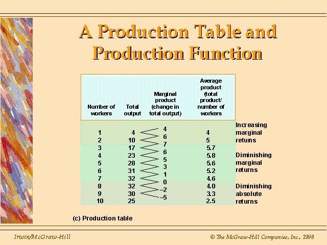
PRODUCTION TABLE: A table that
shows the output produced f/ various combinations of inputs
**********************************************************************************************
EXAMPLE
*in our example we assume inputs are fixed, except for one, labor
we will add the variable input to the fixed
inputs
& see what happens
PRODUCTION FUNCTION:
Is
a graph of the production table information
MARGINAL PRODUCT:
The
additional output produced by an additional input, ceteris paribus
AVERAGE PRODUCT: Total product divided by the variable input
***********************************************************************************************
THE LAW OF DIMINISHING
MARGINAL
PRODUCTIVITY
As more of a variable input is added to fixed inputs, the additional output one gets from the additional input will fall
***********************************************************************************************
TERMS:
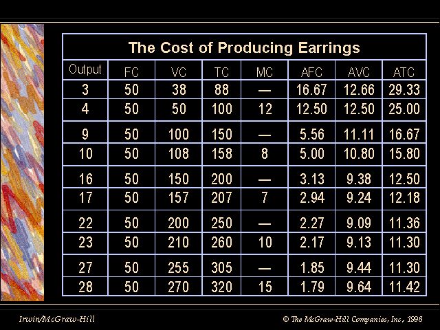
FIXED COSTS (FC): Costs that can not be changed in the time under consideration
VARIABLE COSTS (VC): Costs of the variable inputs; they change as output changes
TOTAL COST (TC): Sum of FC + VC
TC = FC + VC

*to find the average divide by Q (output)
TC = FC + VC = ATC = AFC + AVC
Q
Q
Q
ATC = TC/Q
AFC = FC/Q
AVC = VC/Q
Marginal Costs: cost of increasing output by one unit (MC)
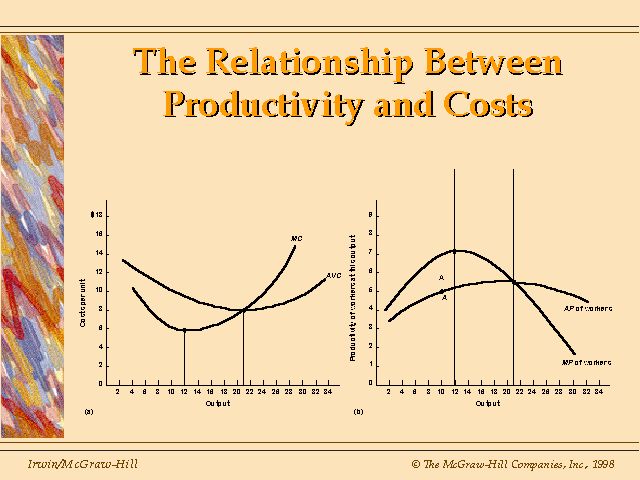
u-shaped MC curve; AVC curve & ATC curve
Initially marginal product increases & costs fall (MC, AVC & ATC). Then "The Law of Diminishing Marginal Productivity" sets in & MP falls forcing costs up (first MC, then AVC and finally ATC).

MC < AVC, then AVC is falling
MC = AVC, then AVC is @ a minimum
MC > AVC, then AVC is rising
MC < ATC, then ATC is falling
MC = ATC, then ATC is @ a minimum
MC > ATC, then ATC is rising
Chapter 9
Supply decisions in the long
run => all inputs are variable
=============================================
Production decisions are based on
Available Technology & Cost
Technical Efficiency: using the least amount of inputs in the
production of a given output
Economic Efficiency:
the lowest cost method of production for a given level
of output
=============================================
production of identical products in different
countries
depends
on the price of inputs
U.S. vs. Mexico => clothes
U.S. vs. China => roads
=============================================
Technical Efficiency is not always Economic Efficiency
this depends on the
level
of output
Indivisible set-up costs:
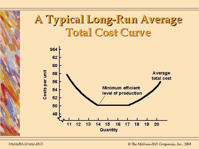
an investment in technology that would only payoff after a MINIMUM
EFFICIENT LEVEL OF PRODUCTION
=============================================
E.G., Pontiac Fiero (200,000) vs. Mazda Miata (30,000)
=============================================
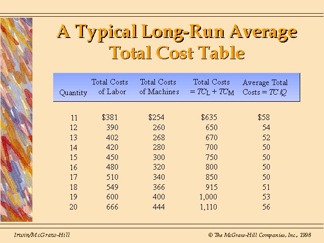
WHAT SHAPES THE LR COST CURVE?
Short-run cost curve is u-shaped because of the law of diminishing marginal productivity
*but in the long run all inputs are variable
Long-run cost curve is u-shaped because of :
1. Economies of scale: cost per unit fall as output rises, e.g., Henry Ford
2. Diseconomies of
scale:
an increase in per unit cost as output rises,
e.g., firm too big
a. Monitoring Cost
b. Team Spirit
Importance of Economies & Diseconomies of Scale
Economies of scale promotes expansion/mergers
Diseconomies promote contraction/takeover defense
Raiders
Real-World Issues:
1. Economies of scope: costs of production are interdependent - costs savings for one product because of producing another. E.G., Purina/Jack-in-the-Box, Pepsico
2. Learn by Doing: firms become more efficient over time w/out any changes in inputs
3. Technological change shifts the cost curve down
4. Unmeasured costs/ accounting vs. economics