Cost Analysis

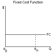
As depicted in the graph to the right, fixed costs are the opportunity costs (implicit and explicit) associated with providing fixed inputs for production. More descriptively, fixed costs are the portion of total cost which are assumed not to vary with the level of output. Examples of fixed costs are the costs involved with warehouse costs, machinery purchase or lease, depreciation of capital assets and contractual commitments. It should be noted that the study of fixed costs is done so over a given range of output. There are no truly fixed costs; instead what we assume to be 'fixed costs' tend to increase incrementally as production increases. For our example fixed cost is depicted as a constant function where the cost at Q₀ is the same at Q_n.

1. As depicted in the graph to the left, variable costs are the opportunity costs (implicit and explicit) associated with providing variable inputs for production. More descriptively, variable costs are the portion of total cost, which vary as production increases. Production of larger quantities of output generally requires relatively larger quantities of particular input. Examples of variable costs include labor, fuel, electricity, and salesperson commissions. In the graph the curve's slope between Q₀ and Q_n1 is increasing at a decreasing rate. This shows that variable costs increase marginally less for each unit added due to greater efficiency or other benefits of greater production to a point. However, at that point (Q_n1) the curve's slope changes and begins increasing at an increasing rate such that every unit added does so at a higher and higher marginal cost. This can be described with the example of there being too many cooks in a kitchen, so much that they become less efficient because of the continual bumping into one another. If the owner wants to increase production, in the long run, we might see an upward shift in the fixed cost curve. This shift would take place if the owner moved his operation to a large facility so that he could accommodate a larger number for workers. In effect he would be moving his variable cost inflection point (the point Q_n1 where marginal cost is zero) further to the right on the graph. In this case we would throw this cost curve out and start again with the new situation. It should be noted here that the difference between fixed costs and variable costs resides in the time horizon assumed. Correctly, in the long run even 'fixed costs' may be changed to suit the needs of production and therefor vary at certain production levels as we see above.

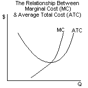
As depicted in the graph to the right, marginal costs are the changes (D ) in opportunity costs (implicit and explicit) associated with providing a one-unit change in output. More descriptively, marginal costs are the addition to the total cost attributable to each additional unit of output. To describe the graph, as the average cost is decreasing per unit the marginal cost is less that the average cost per unit. The marginal cost curve intersects the average cost curve at its minimum. (Marginal Cost = D Total cost/D Quantity produced.)

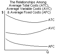
As depicted in the graph to the left, average costs are the opportunity costs (implicit and explicit) divided by the level of output. More descriptively, average fixed costs declines as output increases because fixed costs are independent of production levels. Average variable costs will have a 'U' shape when graphed due to the fact that average variable costs fall as output expands to the point of diminishing returns where the product of one additional input begins to decrease. At that point (the inflection point) the AVC curve will increase. Average total cost is the sum of the average fixed and variable costs. The curve for ATC is downward sloping even past the point where average variable costs begin to slope upward due to the fact that fixed costs decline towards zero thus offsetting the rise in average variable costs to a point where the rise offsets the decline of average fixed costs and the average total costs begins to slope upward. Thus the average total cost curve is also 'U' shaped. It is worth noting in the graph for # 3 that when the average total cost is falling the marginal costs are below the average and when average costs are again increasing the marginal costs are above the average.

Supply

Explicit costs are the part of total opportunity cost which take the form of tangible expenditures on factors of production both fixed and variable. Implicit costs are the portion of total opportunity cost which represent the lost usage of resources from their expenditure on explicit costs. Examples of explicit costs are workers wages, manager's salaries, and hard (e.g. lumber) or soft (e.g. fees for legal advice) resources of production. Implicit cost examples are salaries that could have been earned elsewhere by the firms owners and the use of wholly owned buildings that could be used for something else. Simply put all those costs that show up on the IRS tax report are explicit costs, those that are not represented there are implicit.

Given the above definition of implicit and explicit costs we can differentiate between pure economic profit and accounting profit. Accounting profit is the total revenue less only explicit costs. Pure economic profit is total revenue less both explicit and implicit costs.

Four defining characteristics of perfect competition:

1. Market contains large number of small firms,

2. A homogeneous product,

3. Freedom of entry and exit,

4. Equal access to information.

A "price -taker" is a firm that sells it's output at prices that are determined by forces beyond it's control. A firm that is a price taker perceives a relatively perfect elasticity in it's demand curve at the price level found at the equilibrium of the market supply and market demand curve.

A short-term industry supply curve can be constructed by summing the market's individual firm's supply curve functions. It is important to note that in constructing the industry supply curve that if there was an industry wide move to expand, the shift may cause the price of inputs to increase thus shifting the individual firm's cost curves up. Taking this into account,when we are constructing the industry supply curve over the short term, we would show the final curve steeper than the true sum of the supply curves.

Long run equilibrium for a perfectly competitive market require the following conditions:

The firm must be producing at the optimal productive output for it's individual plant size (short run MC = short run MR)

All firms must individually be satisfied that their plant size is optimal (Short run average total cost = Long run average cost at the minimum on it's curve.)

Incentives for firms to enter or exit the market must be reduced to zero. (Pure economic profit = 0)

Dolan & Lindsey sum these conditions:

Price = MC = Short-run ATC = Long run TC

What these three conditions mean is that if 1) there is internal pressure from the firms individual costs curves to maximize profit it will by moving production in the direction of MC = MR. 2) If there are means that will reduce average total cost and marginal cost by building a different size factory the firm will do that and change the equilibrium. & 3) If firms in the market are operating above 'normal profit' then there will be external market firms wanting to enter thus changing the equilibrium, and subsequently if there are firms making less than 'normal profit' they will be incented to exit the market. Given these conditions we have equilibrium. Moving from these conditions will allow the perfectly competitive market to seek a new equilibrium. Economic profits will always move back to zero.

Perfect competition is perfect in that his maximizes the benefit of price surplus for both the consumer and the supplier. It is can be described further as perfect in that the market-clearing price is the lowest possible price that the right good will be bought or sold.

Perfect competition is not perfect in that firms are at the whims of the wishes of the consumer 100%. The firms engaged are in a constant struggle for survival through reducing costs while trying to produce at 100% efficiency. For all their troubles, due to the ease of entry, the best that any firm can ever hope for in the long run is normal profits (total revenue = implicit and explicit costs).