Graphical Solutions
Improved Euler's Method
Related Websites
Exponential Population Model
Logistic Population Model
Euler's Method
When an exact solution of an initial value problem is not required
or overly complicated, we can often still generate a numerical
solution of the problem.
Such a numerical solution is given by Euler's Method:
Given an initial value problem
the exact solution
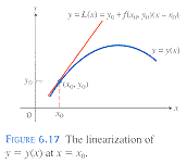
can be approximated by its
linearization
which gives a good approximation
to the exact solution over a short interval.

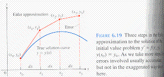
Euler's method is to piece together a string of such linearizations
to approximate the exact solution curve over a longer stretch.
We know
lies on the exact solution curve.
Specify a new value
If the change
gives a good approximation to the exact solution value
The point
lies close to the exact solution curve.
Use the point to get the next approximation
and then use this point to get the next approximation
and so on.
We approximate the exact solution curve by a sequence
of straight lines that lie very close to the exact solution curve.

See Example 1 - 2, pages 509 - 511.
Graphical Solutions
Plot the data pairs in a numerical solution to visualize the
approximate solution.
See Example 3, page 511.
Improved Euler's Method
The method can be improved by taking the average of two slopes.
See Example 4, page 512.
Exponential Population Model
A common model of population growth is to assume that the
population
for some constant
The solution is
where
is the size of the population at time
The ratio
is called the relative growth rate.
See Example 5, pages 513 - 514.
Logistic Population Model
The exponential model for population growth assumes unlimited
growth and that the relative growth rate is constant.
That is not always the case.
See Table 6.9, page 514.
A more refined description of population growth is given by the
logistic growth model
where
that the environment is capable of supporting.
See Example 6, pages 515 - 517.
next Hyperbolic Functions
Top