Separable Equations and Solution
Slope Fields:Viewing Solution Curves

Examples of Differential Equations
         in Applications:
Law of Exponential Change
Continuously Compounded Interest
Radioactivity
Heat Transfer: Newton's Law of Cooling
Resistance Proportional to Velocity
Torricelli's Law


             First-Order Separable Differential Equations

A first-order linear equation

is separable if   can be written as the product of a function of 
and a function of  .
In other words, the equation has the form
.
If   , we can separate the variables by dividing
both sides by  ,

.

Integrate both sides


or
.
With the   and   separated, one on side of the equation
and the other on the other side, we integrate and complete
the solution. That is the basic process for solving a separable
linear first-order differential equation.

See Example 2, pages 486 - 487.


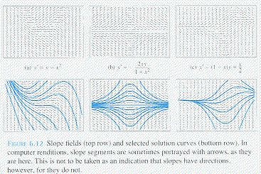
Slope Fields: Viewing Solution Curves
Because the general solution of the differential equation 

contains an arbitrary constant, the graph of the solution
consists of an infinite of curves.
Graphing the equation

directly associates to each point (within the domain of   ) a slope.
Such a graph is called a Slope Field.




             Examples of Differential Equations in Applications

Law of Exponential Change
Examples of phenomena where a quantity   increases or decreases
at a rate proportional to the amount present are population, radioactive
decay, continuously compounded interest, and heat transfer.
The phenomena may be represented mathematically by the
differential equation

with the initial condition
.
The derivative is taken with respect to time .
The solution of the initial value problem is
,
where    represents growth and    represents decay.
The number
   
is the rate constant of the equation which characterizes
the specific context of the phenomenon in question.


Continuously Compounded Interest
Suppose

dollars are invested in an account in which the interest is added continuously
- that is, at every moment of time, not just annually or quarterly -
then we can model the growth of the account with the initial value problem

,
whose solution is
.
The number

is the continuous interest rate.

See Example 3, page 489.


Radioactivity
The decay of a radioactive element is described by
,
.
  is the amount of the radioactive substance at time zero.
The amount still present at at a later time  will be
.
The half-life of a radioactive element is the time required for half
of the radioactive nuclei present in a sample to decay.

See Examples 4 - 5, pages 489 - 491.


Heat Transfer: Newton's Law of Cooling
Study a heated object immersed in a cooler surrounding medium.
The object, in time, will cool down to the temperature of the surrounding
medium and the differential equation describing this process is
,
where 
 
is the temperature of the object at time 
and 

 is the constant surrounding temperature.
If we let
,
 the above equation becomes
.
We have seen this basic equation many times before!
Its solution is
,
where

and    is the temperature at .
Returning to the original symbols, Newton's Law of Cooling is then

.

See Example 6, pages 491 - 492.


Resistance Proportional to Velocity
Imagine an object of mass   moving along a coordinate line with its
position and velocity at time   given by   and  , respectively.
By one of Newton's Laws of Motion
                                                         Force = mass times acceleration
the force resisting the motion can be written as
.
The condition that the resisting force is proportional to the velocity
can be written as

or
.
If the sign in the differential equation were positive instead of negative,
the force would be assisting the motion, not resisting it.

Its solution with initial condition

is
.

See A Moving Body Coasting to a Stop and Example 7, pages 493 - 494.


Torricelli's Law
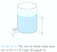
If you drain a tank like the one pictured below, the rate at which
the water runs out is a constant times the square root of the water's depth  .
The constant depends on the size of the exit value.


See Example 8, pages 494 - 495.


          next      Linear First-Order Differential Equations
                      Top