|
|
|
|
Sources for 1/f noise effects in human cognition
and performance
Jeffrey Pressing
Department of Psychology
University of Melbourne
Parkville, Vic. Australia 3052
E-mail: jeff@intelligenesis.net
Abstract
1/f noise is a widespread phenomenon in physical and behavioral systems.
It typically occurs in systems that show long-term memory, and its sources
are likely to be multifarious. This paper shows how a modeling approach
which combines moving averages of 2 or more distinct time scales readily
yields 1/f-type noise spectra. This result is then interpreted psychologically,
suggesting that recent extensive findings of 1/f noise in human behavior
may well result from the presence of attentional, memory or control structures
operating on distinct time scales, for which there is considerable evidence.
Also presented is an alternative autoregressive modeling approach, which
is shown to only yield 1/f type spectra under rather special conditions
and hence does not provide a route of general explanation.
Key words: 1/f noise, moving average, power spectrum, time scale,
model
Introduction
"1/f noise" refers to a relation between a system's spectral
power density ![]() and its frequency
and its frequency ![]() of
the form
of
the form ![]() , with beta about
1. Thus a log-log plot of S &
, with beta about
1. Thus a log-log plot of S & ![]() will be linear with slope
will be linear with slope ![]() , where beta is near 1 (in practice, it may vary as widely as 0.51.5 or
2).
, where beta is near 1 (in practice, it may vary as widely as 0.51.5 or
2). ![]() noise occurs widely
in physical systems such as semiconductors, superconductors and optical
devices (e.g., Handel & Chung, 1993). Recent work (Gilden et al., 1995;
Gilden, in press, Pressing & Jolley-Rogers, 1997) has found evidence
for 1/f noise in various human estimation tasks, including tapping,
line drawing, and spatial sectioning of line segments. Such effects have
also been found in a variety of sequential reaction time measurements of
cognitive processes: mental rotation, lexical decision, serial visual search,
and parallel visual search (Gilden, in press). In a related paper, Wing
& Pressing (in preparation) have found such effects in force production
tasks. After illustrating the nature of the effect, this paper is concerned
with simulations that allow the inference of mechanisms responsible for
it and an elucidation of possible relations between experimental manipulations
and spectral exponent value (that is, beta in the
noise occurs widely
in physical systems such as semiconductors, superconductors and optical
devices (e.g., Handel & Chung, 1993). Recent work (Gilden et al., 1995;
Gilden, in press, Pressing & Jolley-Rogers, 1997) has found evidence
for 1/f noise in various human estimation tasks, including tapping,
line drawing, and spatial sectioning of line segments. Such effects have
also been found in a variety of sequential reaction time measurements of
cognitive processes: mental rotation, lexical decision, serial visual search,
and parallel visual search (Gilden, in press). In a related paper, Wing
& Pressing (in preparation) have found such effects in force production
tasks. After illustrating the nature of the effect, this paper is concerned
with simulations that allow the inference of mechanisms responsible for
it and an elucidation of possible relations between experimental manipulations
and spectral exponent value (that is, beta in the ![]() relation).
relation).
1/f noise in force production
In work reported fully elsewhere, Wing & Pressing (in preparation) measured grip force and load force for a repeated vertical force task. The task was to perform iterated vertical force pulses using a thumb vs forefinger and middle finger grip on a solid metal circular cylinder, using one of two learned force levels, and at one of different speeds. The runs were executed in continuation mode, so that a computer-generated tone indicated the correct approximate tempo initially for 8 trials; thereafter, the tone ceased. The forces at each regular force peak were then determined by a peak detection algorithm, and their sequential values formed the time series used in analysis. In this work we found consistent clear examples of 1/f noise. Two examples of this from the pilot study are found in figures 1 & 2.
Figure 1 shows the load (vertical) force for one subject performing at about 300 ms period, with a 200 Hz sampling rate and run length of 600 events. Figure 2 shows the grip (horizontal) force for the same run for the same subject. Both plots show classic 1/f linearity.
These graphs are typical of the results in psychological experiments, in that linearity is found for low to medium values of frequency, and there is often a (typically short) plateau for the high frequencies.
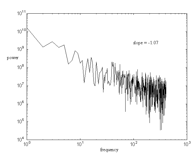
Figure 1: load force spectral power density for a single run
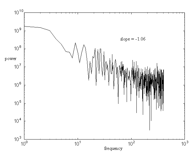
Figure 2: grip force spectral power density for a single run
An investigation of theoretical underpinnings
We seek to identify simple mechanisms for the 1/f effect. Although
there appears to be no universal analytical procedure that generally explains
all cases of ![]() spectral forms,
several types of system structure have been been found to yield such behaviour.
spectral forms,
several types of system structure have been been found to yield such behaviour.
One perspective on 1/f processes ascribes them to self-similarity across different levels of system structure. This fractal property shows itself in the fact that the sum or product of two 1/f processes is 1/f (Kawai, et al., 1993), and in the absence of a characteristic distance or time scale, a phenomenon known as scale invariance. Since exact self-similarity is not essential, one pragmatic and easily modelled form of this perspective is the idea that 1/f spectra can arise from systems that feature multiple discrete time scales (e.g., in relaxation or processing or production), or certain continuous distributions of them (Montroll & Shlesinger, 1982). From this perspective, nonlinearity and determinism play no essential role (Handel & Chung, 1993). Multiple time scales have been been invoked as explanations of human cognitive control processes and attentional fluctuations (e.g., Pressing & Jolley-Rogers, 1997), and simulations based on this approach are presented as Method 1 below.
Another perspective is that 1/f spectra are associated with certain
conditions of deterministic nonlinearity. Thus, such spectra are found
to occur in many cases where deterministic nonlinear systems operate either
in intermittency or chaotic regimes (Handel & Chung, 1993; Shuster,
1996), although such outcomes are certainly not universal. (The intermittency
case provides a clear link with the idea of multiple time scales, because
intermittency always yields at least 2 time scales.) Handel (1993) has
shown that nonlinear state equations with a homogeneous characteristic
function are necessarily 1/f when operating in the chaotic regime.
This result applies to both classical and quantum mechanical models of
physical systems. Thus instability or marginal stability is an essential
element in this perspective. Hence below, with Method 2, we look at (linear)
systems operating on the cusp of autoregressive stability.
Method 1
The first simulation method begins with an uncorrelated white noise
process ![]() . One simple way
to generate multiple time scales from such a process is to use a moving
average operation. Let us denote the moving average of
. One simple way
to generate multiple time scales from such a process is to use a moving
average operation. Let us denote the moving average of ![]() based on a time window of
based on a time window of ![]() points by
points by ![]() . That is, the
nth term of
. That is, the
nth term of ![]() is
just
is
just
![]() , so
that (1)
, so
that (1)
a simple example of a 3-time scale process would be
![]() , (2)
, (2)
which invokes the time scales 1, ![]() and
and ![]() . Here
. Here ![]() and
and ![]() are weights for the
moving average processes. Two actual series produced in this way are shown
in figures 3a & 3b.
are weights for the
moving average processes. Two actual series produced in this way are shown
in figures 3a & 3b.
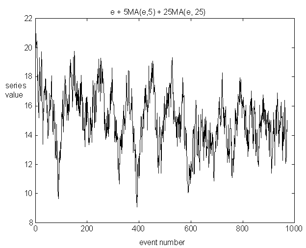
Figure 3a: sample time series with three time scales (1/f slope = -1.26)
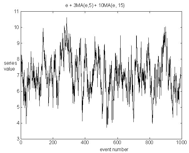
Figure 3b: a second sample time series with three time scales (1/f slope = -1.05)
Equations of the type (2) readily generate 1/f-like shapes. Three examples are shown in figures 4a, 4b, & 4c for single runs of 1024 points, using a white noise source with a uniform distribution over [0,1].
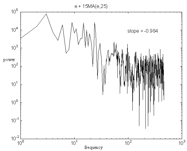
Figure 4a: spectral power density of white noise plus one moving average of white noise
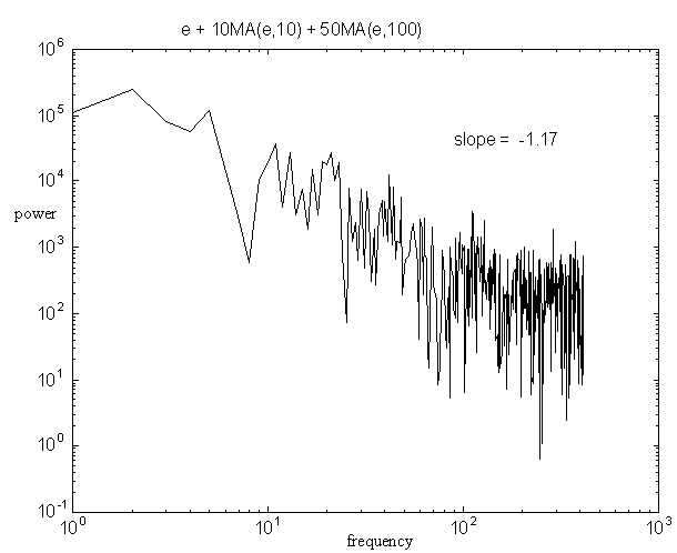
Figure 4b: spectral power density of white noise plus two moving averages of white noise
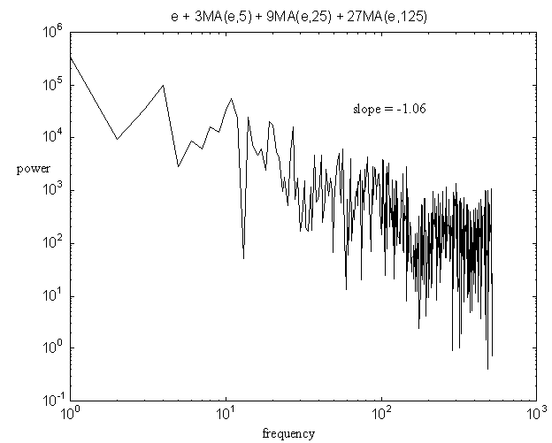
Figure 4c: spectral power density of white noise plus three moving averages of white noise
Figures 4a, 4b, & 4c respectively show 2, 3, and 4 time scales. Slopes were determined from a simple linear best fit. The three figures illustrate the qualitative results of a considerable number of simulations, which suggested two things: three processes (figure 4b) give a more nearly linear plot than two (and there is perhaps an additional smaller improvement with four processes); and the precise values of weights and time windows do not greatly alter the property of approximate linearity or the value of the exponent, provided long time scale terms have greater weights.
In the time domain, 1/f processes are associated with long range autocorrelation. Figure 4d shows a sample correlogram of the 4 time scale process of figure 4c. The general fall off to zero over the range of the largest moving average is typical, but repeated simulations show considerable variability, and in many cases the trend to zero is far from monotonic.
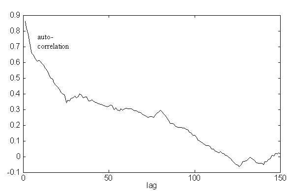
Figure 4d: example of a correlogram of the 4 time process of figure 4c.
The effects of weights and times on slope can be demonstrated more systematically
by a series of simulations using three time scales in which we set ![]() and
and ![]() . This means that the
time windows can be considered to be based on a single scale factor
. This means that the
time windows can be considered to be based on a single scale factor ![]() and the weights can be considered to be based on a single scale factor
and the weights can be considered to be based on a single scale factor ![]() ,
and that we factor in a certain degree of self-similarity. The explicit
form of the series is thus
,
and that we factor in a certain degree of self-similarity. The explicit
form of the series is thus
![]() (3)
(3)
We determined the ![]() power
spectral density log-log slopes over the ranges
power
spectral density log-log slopes over the ranges ![]() and
and ![]() , with the results
as in figure 5.
, with the results
as in figure 5.
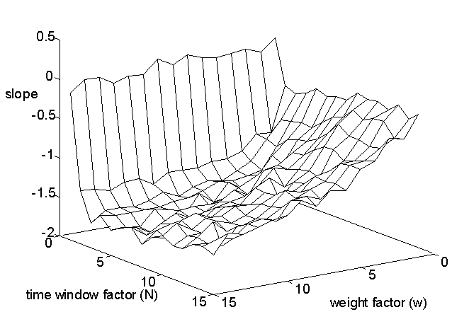
Figure 5: log-log 1/f slopes for a sum of three sources: white noise, and two weighted moving averages of white noise. See Eq. (3). Factor ranges are 115 in both cases.
Each of the 225 points represents a 1000 event simulation with the indicated time window and weight factors. The results show that when the time window factor is 1, the spectral power density gives a slope near zero, as it should, since in this case we have white noise at a single time scale. However, inclusion of processes with time window greater than 1 causes the slope to drop markedly. Over the entire range of time window and weight factors, the slope is primarily between -0.5 and -1.5. The average slope for all 225 points is -1.087. Weight factors in the range 46 were found most likely to yield slopes close to -1. There is, of course, no guarantee that such values are optimum in other systems. However, similar results were obtained with the same range of factors for two and four time scales.
For time window factors greater than 1, the time window size factor
has a relatively weak effect overallsee figure (5). The direction of the
effect can be seen in the following figure 6, which roughly corresponds
to a view from the left in the previous figure of a slice of the surface
made by a plane parallel to the time window/slope plane, although here
the time factor is the scale of the longest window, not a ratio between
both time window lengths. Since this factor has the largest weight, the
effect is amplified over that seen in figure 5:
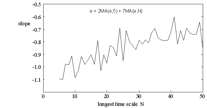
Figure 6: spectral power density slopes for various longest time scales
Each point here is a 1000 event run with slope produced by simple linear fitting.
On the basis of these simulations it appears that the primary determinant of the slope is weight factorthat is, the relative strength of the different components, with less effect from their particular time values. This can be interpreted as meaning that 1/f noise effects point to processes operating at different time scales and with markedly different amplitudes.
This result shows that fractal like structure in time can indeed produce 1/f behaviour, and that neither deterministic causation nor nonlinearity is required to do so. The high frequency plateau occurs because at the very highest frequencies only effects from the single fastest frequency will be significant, creating a within-band approximation to white noise, hence, a noisy plateau. In other frequency ranges, at least two time scales interact. Further examination of simulations supported this point, so that when the time scale factor was large, the size of the high frequency plateau increased, at the expense of the region of linearity.
This general trend can be shown quantitatively. Simulations were performed with a weight factor of 5, and time window factors varying from 2 to 15. In each case, 5 runs of 1024 points were run, and an estimate of the high frequency plateau size determined as follows: First the moving average of the power spectral density was computed with a window of 6 bins. Then the point of lowest frequency that was still <= 10% above the mean power value of the highest 100 frequency bins (412-511) of the moving average was determined, call it bin Z. Then plateau size was estimated as plateau size = ln(511) - ln(Z). The result is shown in figure 7. Error bars indicate standard errors.
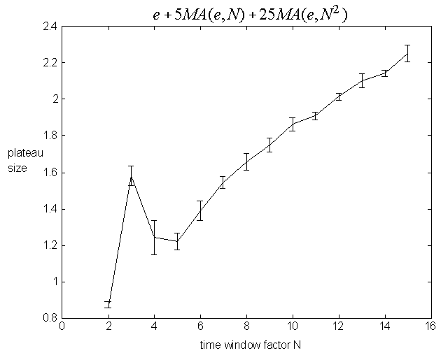
Figure 7: An illustration of increase in high frequency plateau size with time window factor N.
Method 2
Another method that can produces linear log-log spectral plots is based on a simple linear autoregressive model. Consider a 2nd order ARMA-like model (Pressing, 1997) with parameters alpha and beta.
![]() (4)
(4)
Here alpha and beta are respectively first and second order error correction
parameters, and the other variables (![]() )
are white noise sources with P = mean (C).
)
are white noise sources with P = mean (C).
For nearly all values of alpha and beta, this autoregressive model yields
a flat spectrum of slope about zero. However, consider the special case
when beta is equal to minus alpha. In this case the model is only marginally
stable, since for alpha + beta < 0, the model is unstable. Hence the
model is on the threshold or cusp of stability. When alpha = beta = zero,
the process is a random walk (with a modified noise structure), which is
known to yield ![]() , or Brownian
noise.
, or Brownian
noise.
Simulations were performed under this condition, varying the alpha (and
hence negative beta) parameter in increments of .1 from -1 to +1. Outside
this range the series is unstable. Parameter values for the Gaussian white
noise sources were those typical of human performance of rhythmic temporal
patterns: mean(C) = P = 500 ms, sigma(C) = 15 ms; mean(M) = 40 ms, sigma(M)
= 3.5 ms. Figure 8 shows the first 1000 points of a typical single run
and figure 9 shows a power spectrum plot for the same run, which had ![]() .
Deviations from linearity at the highest frequencies are pronounced, but
if this range were not measured, or reduced in power by filtering, a very
good linear plot would be the result.
.
Deviations from linearity at the highest frequencies are pronounced, but
if this range were not measured, or reduced in power by filtering, a very
good linear plot would be the result.
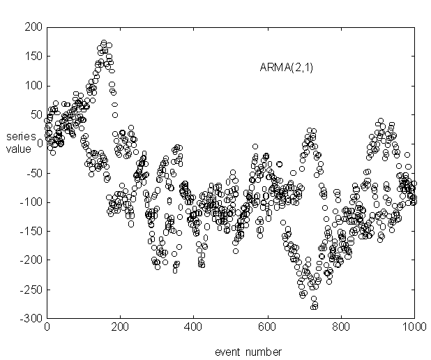
Figure 8: an ARMA-like time series from Eq (4) in a region of marginal
stability, with ![]()
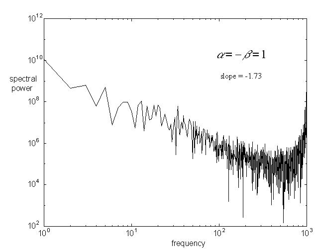
Figure 9: power spectrum for the series of figure 8
The generality of this was examined as follows: At each alpha value 10 runs of individual length 2048 points were obtained. Resultant slopes were averaged over the 10 runs and figure 10 shows the results in plot of slope versus parameter. All plots had extended regions of linearity with negative slope. Some plots showed a limited plateauing or increase effect for high frequencies. Therefore the best linear slope was computed for bins 1500 (a large fraction of the range on the log-log plot) so that the nonlinear portion of the curve did not bias the apparently linear portion for lower frequencies. If this restriction was not imposed, then some slopes moved into the upper reaches of the 1/f region as before.
Each point in the graph represents the results of 10 runs of 2048 steps per data point. Error bars indicate standard errors.
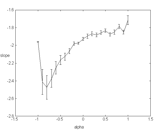
Figure 10: Slope of best linear fit for low frequency linear region in a log-log plot of spectral power density vs. frequency as a function of autoregressive parameter alpha
Conclusions
The work here confirms that the presence of multiple time scales can credibly yield 1/f noise effects over a wide parameter range. Marginal stability regimes can yield negative power spectrum slopes as well, but slopes are generally considerably more negative than minus one and may show high frequency peaking. The results here do not yield unique identification, since other types of system behaviour can yield 1/f effects: for example, the important theory of extremal events of Miller, Miller, and McWhorten (1993). However, the mechanism of multiple time scales has in its favour both physiological and psychological plausibility when we are looking in the domain of human behaviour.
The main points found were:
summed effects of multiple time scale random processes can naturally yield 1/f spectra, with exponents mainly in the range -1.5 to -.5 when fractal scale factors vary over the range 215
many time scales are not required; 3 or even two is sufficient
to achieve 1/f effects, slow processes must have greater amplitude (weight) than faster processes
the power spectrum exponent is more affected by process weight than process time scale factor
power spectrum exponent increases (becomes less negative) with decreasing weight factor
power spectrum exponent increases (becomes less negative) with increasing time scale factor
size of high frequency plateau tends to increase with time scale factor
goodness of fit to a straight line tends to increase with number of processes
What are the specific sources of such processes in the organism? These
are not difficult to imagine. At the neurophysiological level, neural interactions
acting over various distance scales, and based on different local capacities,
efficiencies and task requirements, will clearly tend to produce mutiple
time scales and amplitudes. At the behavioral level, common experience
teaches that overt behaviours organized around a particular goal or set
of linked goals operate over various time scales. At the cognitive level,
two obvious candidates are attention and memory. Memory is customarily
divided into three time scales: that of the sensory store, that of short
term memory, and that of long term memory. Likewise, different time scales
play a role in standard classifications of attention, as automatic, conscious,
or sustained. Vigilance tasks, with which the tasks here have a considerable
amount in common, typically exhibit drifts of attentional focus over various
time frames, with larger deviations occurring with larger time scales.
Acknowledgment
This work was produced with the assistance of a grant from
the Australian Research Council.
References
Gilden, D. L., Thornton, T., & Mallon, M. W., (1995) 1/f noise in human cognition? Science 267, 1837-1839.
Handel, P. H. (1993). The nature of fundamental 1/f noise. in P. Handel & A. Chung (Eds.), Noise in physical systems and 1/f fluctuations. pp 162171.
Handel, P. H., & Chung, A. L. (Eds.) (1993). Noise in physical systems and 1/f fluctuations. New York: American Institute of Physics.
Kawai, T., Mihira, Y., Sato, M., & Hayashi, M. (1993). Basis of universal existence of 1/f fluctuations. in P. Handel & A. Chung (Eds.), Noise in physical systems and 1/f fluctuations. pp. 639642.
Miller, S. L., Miller, W. M., and McWhorten, P. J. (1993). Extremal dynamics: A unifying physical explanation of fractals, 1/f noise, and activated processes. Journal of Applied Physics, 73(6), 2617.
Montroll, E. W., & Shlesinger, M. F. (1982). Proceedings of the National Academy of Sciences, 79, 3380.
Pressing, J., & Jolley-Rogers, G. (1997). Spectral properties of human cognition and skill. Biological Cybernetics, 76(5), 339-347.
Schuster, H. G. (1996). Deterministic chaos: an introduction. Cambridge: Weinheim.
Wing, A., & Pressing, J. (in preparation) . The variability of force control in human motor skill.