PURPOSE: To use ds9 software to analyze the X-ray spectrum of the Tycho Supernova Remnant, determine the elements present, and investigate the distribution of these elements in the remnant.
TARGETS:
Benchmarks/Project 2061:
4a. Increasingly sophisticated technology is used to learn about the universe. Visual, radio, and x-ray telescopes collect information from across the entire spectrum of electromagnetic waves; computers handle an avalanche of data and increasingly complicated computations to interpret them; space probes send back data and materials from the remote parts of the solar system; and accelerators give subatomic particles energies that simulate conditions in the stars and in the early history of the universe before stars formed.
Mathematical models and computer simulations are used in studying evidence from many sources in order to form a scientific account of the universe.
Maine Learning Results:
G1. Describe how scientists gather data about the universe.
L7. Use computers to organize data, generate models, and do research for problem solving.
PRIOR KNOWLEDGE:
Students should be familiar with the electromagnetic spectrum, emission spectra, stellar evolution, and element formation in stars and supernovae.
INTRODUCTION:
 Fig. 1 Tycho Brahe |
 Fig. 2 Stella Nova |
On the evening of November 11, 1572, Danish astronomer Tycho Brahe noticed a new, very luminous object in the constellation Cassiopeia. This object became bright enough (as bright as Venus!) to be observed for several weeks during the day. Over the next year and a half, it dimmed by a factor of about 10,000 until it was no longer visible to the naked eye, even at night.
“If it were a star, then the immutable heavens had changed, and the basic contrast between the superlunary region and the corruptible earth was in question. If it were a star, the earth might more easily be conceived as a planet, for the transitory character of terrestrial affairs would now have been discovered in the heavens as well. Brahe and the best of his contemporaries did conclude that the visitor was a star. Observations … indicated that it could not be located below the sphere of the moon or even close to the sublunary region. Probably it was among the stars for it was observed to move with them. Another cause for cosmological upheaval had been discovered.“
~from The Copernican Revolution, Thomas Kuhn
Tycho’s “Stella Nova”, however, was not the birth of a star as he had thought, but the death of a star or a supernova.
BACKGROUND INFORMATION:
A light curve reconstructed from Brahe’s observations has shown that this supernova is a Type 1a. A star can have different fates depending upon its mass. A star with about the same mass as the Sun will turn into a white dwarf. If this white dwarf is in a binary system, it can accrete enough mass so that it cannot support its own weight. The star collapses and temperatures become high enough for carbon fusion to occur. Fusion begins throughout the white dwarf almost simultaneously and an explosion occurs.

Fig. 3 Supernovae light curves


Fig. 4 White Dwarf in a Binary System, Tycho's SNR
NASA's Chandra X-ray Observatory, which was launched and deployed by the Space Shuttle Columbia on July 23, 1999, is the most sophisticated X-ray observatory built to date. Incoming X-rays are focused by the mirrors to a tiny spot (about half as wide as a human hair) on the focal plane, about 30 feet away. The focal plane science instruments, ACIS and HRC, are well matched to capture the sharp images formed by the mirrors and to provide information about the incoming X-rays: their number, position, energy and time of arrival. Two additional science instruments provide detailed information about the X-ray energy, the LETG and HETG spectrometers.
ds9 software (available as a free download from the Chandra Ed website) allows educators, students, amateur astronomers and the general public to perform X-ray astronomy data analysis using data sets from the Chandra X-ray Observatory. Let’s look at Tycho’s SNR!

Fig. 5 Chandra X-ray Observatory
| HYPOTHESIS – write this on
your lab
sheet. Use prior knowledge about stellar evolution to make predictions about the elements you might expect to see in a Type 1a supernova remnant and how those elements might be distributed in the remnant. What elements would you expect to find? Where would the heavier elements be found in the remnant? Where would the light elements be? Explain your reasoning. You may wish to read more about the X-ray spectroscopy of SNRs here before making your hypothesis. |
 Fig. 6 Cross-section of a white dwarf |
Install the software and load the FITS file (data/image file):
1. Download and install ds9 according to the instructions on the Chandra-Ed web site.
2. Open ds9. From the menus, choose Analysis>Virtual Observatories>Chandra-Ed Archive Servers.
3. Click “Obs ID 115 – ACIS OBSERVATIONS OF TYCHO AND KEPLER”.
4. Under the “Color” menu, choose the color that shows the most detail for you.
5. As you complete this activity, document your investigation by taking screen shots of each step of your ds9 analysis (use the Print Scrn button on the keyboard) and then pasting them into a PowerPoint or Word document. Number these screen shots and write notes about what you were doing and/or observations for each one on your lab sheet or type them directly into the document containing your screen shots.
Plot the spectrum of Tycho’s SNR:
6. Click in the center of the Tycho SNR and drag a circular region around it.
7. Choose Analysis>Chandra Ed>CIAO:Sherpa Spectral fit.
8. For “Model Type”, choose “bremsstrahlung”.
9. On the graph window that comes up, choose Graph>linear-log.
WHAT IS BREMSSTRAHLUNG?
 Fig. 7 Bremsstrahlung |
A supernova remnant can have a temperature of millions of degrees Kelvin. Bremsstrahlung radiation occurs in such a hot gas where many electrons are stripped from their nuclei, leaving a population of electrons and positive ions. When an electron passes close to a positive ion, the strong electric forces cause its trajectory to change. The acceleration of the electron in this way causes it to radiate electromagnetic energy - this radiation is called bremsstrahlung and produces a continuous X-ray spectrum. |
In addition, emission lines can appear superimposed on this spectrum, corresponding to the ejection of K and L shell electrons knocked out of atoms by collisions with high-energy electrons. Higher energy electrons then fall into the vacated energy state in the outer shell, and so on, emitting X-ray photons. The energies of these emissions lines can be matched to energies in the CHIANTI Atomic Database to identify the elements in plasmas such as supernova remnants.
Identify the emission lines in Tycho’s SNR:
10. Enlarge the graph by dragging the lower right corner or clicking the maximize square. To print the graph, use the Print Scrn button on the keyboard and then paste the graph into a program such as Powerpoint or Word and print it from there.
11. To get the energy of each emission line, create a zoom box on the graph by holding the left mouse button down and dragging a box around the area of the emission line. When you click again, a zoom will appear. Right clicking the mouse returns you to the original graph. (See Fig. 8)


Fig. 8 Zooming in on an emission line
12.An alternative way of getting the energy of each emission line by using your printout from #10 is to measure the distance between 1 and 2 keV to the nearest tenth of a centimeter (mm). This gives your scale in cm/keV. Measure the distance in cm (to the nearest 1/10 cm) from 1 keV to the center of each peak (X- ray emission line).
13. Divide the distance to each peak (cm) by your scale (cm/keV) and add 1 KeV to get the energy (keV) of each emission line.
14. Record the energies and identify the elements for each
X-ray emission line/peak using this table. If you have lines whose energy
is not close to that of one of the elements in the chart, leave that line
unidentified.
15. You may wish to use the CHIANTI database to get possible candidates for
unidentified lines. You will need to convert energies in KeV to
wavelengths in angstroms using E = hc/l where h = 6.626X10⁻³⁴ js, c = 3 X 10⁻⁸
m/s, 1A = 1.6 X10⁻¹⁰ m and 1 keV = 1.6 X10⁻¹⁶ j. This gives you the formula:
Energy cuts – distribution of elements:
16. Choose Analysis>Display Contours. This makes a contour map of photon counts. The contour lines are green and show up better on some color schemes than others.
17. If you wish to see the contour intervals – Analysis>Contours Parameters.
18. Use Analysis>Chandra Ed Analysis Tools>Energy Cut to view the Tycho SNR in an energy band close to the energy values of the emission peak for each element (choose a hi and lo of 0.1KeV on either side of the line energy). Click “display all images in tile mode”. Energy cuts will help you see the distribution of the elements. Analysis>Display Contours is useful here. Label your screen shots with the appropriate element and the energy range (See Fig. 9) or record this on your lab sheet. IMPORTANT - before making an energy cut, make sure you click on the frame with the original picture.
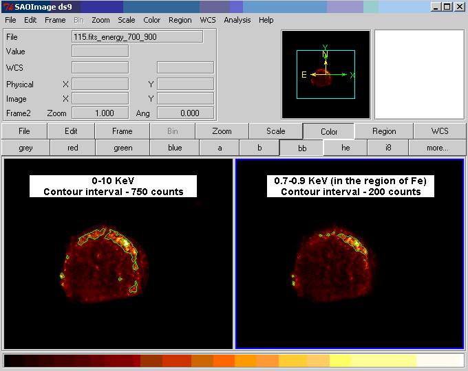
Fig. 9 Energy Cut in the range of the 0.8 KeV iron emission line
19. On your bremsstrahlung spectrum, there is an energy continuum where there are no spectral lines. Do an energy cut for this energy interval. Think about what this area might represent and why there are no spectral lines in this region.
Spectra of various regions in Tycho’s SNR:
20. Scientists are often interested in the composition of specific areas of a supernova remnant such as a knot that is very rich in a certain element. Using various shaped regions (box, polygon, circle, etc – click the “Region” button on the task bar and then “more” to see the available shapes or use the pull-down menu Region>Shape), enclose areas of interest from your energy cuts and create bremsstrahlung spectra as you did for the whole Tycho SNR. Leave your graph axes as linear-linear. If you position your spectrum plot as shown in Fig. 10, you can make a screen shot that shows both the plot and the area you enclosed. Can you find a knot that is very rich in iron?

Fig. 10 Spectrum of a selected region of Tycho’s SNR
CONCLUSIONS:
1. What elements did you identify and how were they distributed within the remnant? Do the results of your ds9 analysis support your hypothesis? Why or why not?
2. How do the spectra of different regions you investigated within the Tycho SNR compare to each other? What are their similarities and differences?
3. Describe the shape of the region for the energy cut of the continuum that contained no spectral lines. What could this represent? Why doesn’t it contain spectral lines?
4. Describe the features and shape of the Tycho SNR.
REFERENCES:
X-Rays - Another Form of Light
X-ray Sources: Supernovas & Supernova Remnants
Chandra's View of Tycho's Supernova Remnant
Chandra Education Data Analysis Software & Activities
XMM-Newton observation of the Tycho Supernova Remnant
Chandra Observations of Tycho's Supernova Remnant
Chandra Images by Category - Supernovas & Supernova Remnants
Chandra Supernova Remnants Catalog
Universe Today - Survivor Found From Tycho's Supernova
*Special thanks for assistance
with the development of this project to Dr. Frederick Seward of the Smithsonian
Astrophysics Observatory.