Principle Foundations      Home Page

Simple Regression Analysis

THE TWO-VARIABLE LINEAR MODEL

(bivariate model)

     Simple regression is used for testing hypothesis about the relationship between a dependent variable, Y, and and independent or explanatory variable, X, and for prediction. This is to be contrasted with multiple regression analysis, in which there are not one, but two or more independent or explanatory variables.

Linear regression analysis assumes that there is an approximate linear relationship between X and Y (i.e. the set of random sample values of X and Y fall on or near a straight line). This is to be contrasted with non-linear regression analysis.

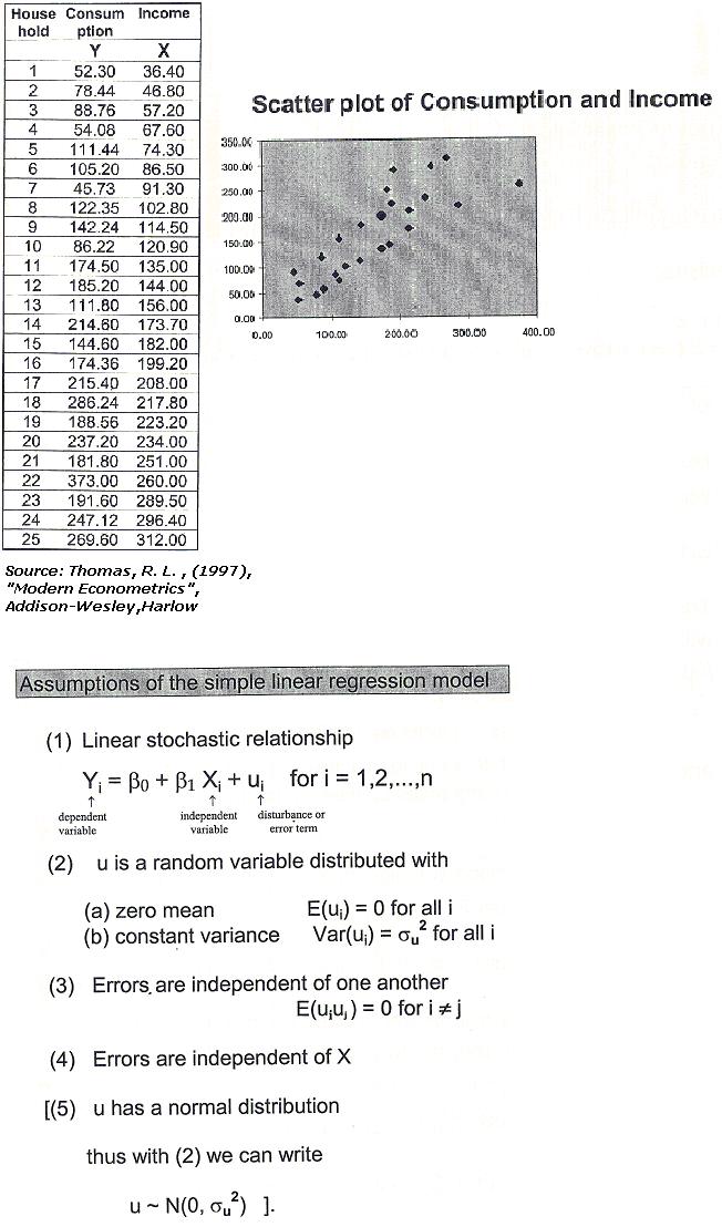
A scatter diagram is a figure in which each pair of independent - dependent observations is plotted as a point in the XY plane. Its purpose is to determine (by inspection) if there exists an approximate linear relationship between the dependent variable, Y, and the independent or explanatory variable, X.

• numerous explanatory variables with only slight and irregular effects on Y that are omitted from the exact linear relationship given by Eq.(1.5), 
• possible errors of measurement in Y, and 
• random human behavior.

The two-variable linear model, or simple regression analysis, is used for testing hypotheses about the relationship between independent variable, Y, and an independent or explanatory variable, X, and for prediction. Simple linear regression analysis usually begins by plotting the set of XY values on a scatter diagram and determining by inspection if there exists an approximate linear relationship.

                                    Y_i = b₀ + b₁X_i                                    (1.5)

Since the points are unlikely to fall precisely on the line, exact linear relationship in Eq.(1.5) must be modified to include a random disturbance, error, or stochastic term, u_i :

                                    Y_i = b₀+b₁X_i+u_i                                  (1.6)

The error term is assumed to be ;

• normally distributed,

• with zero expected value or mean

• constant variance, and it is further assumed 

• the error terms are uncorrelated or unrelated to each other

• the explanatory variable assumes fixed values in repeated sampling (so that X_i and u_i are also uncorrelated).

Example: 

For a given level of the independent variable (X_i=income), the expected level of the dependent variable (Y_i=consumption) will be:

E(Y_i/X_i)=β₀+β₁X_i

  Assumptions of the classical linear regression model (OLS):

• The first assumption is that the random error term u is normally distributed. As a result, Y and the sampling distribution of the parameters of the regression are also normally distributed, so that tests can be conducted on the significance of the parameters.

• The second assumption is that the expected value of the error term or its mean equals zero: that is 

E(u_i) = 0

Because of this assumption, Eq (1.5) gives the average value of Y. Specifically, since X is assumed fixed, the value of Y in Eq (1.6) varies above and below its mean as u exceeds or is smaller than 0. Since the average value of u is assumed to be 0, Eq (1.5) gives the average value of Y.

• The third assumption is that the variance of the error term is constant in each period and for all values of X; that is               

E(u_i)² = .

This assumption ensures that each observation is equally reliable, so that estimates of the regression coefficients are efficient and tests of hypothesis about them are not biased. These first three assumptions about the error term can be summarized as 

u ~ N(0, )

• The fourth assumption is that the value which the error term assumes in one period is uncorrelated or unrelated to its value in any other period; that is,

E(u_iu_j) = 0        for       ; i,j = 1,2,….,n 

This ensures that the average value of Y depends only on X and not on u, and it is once again required in order to have efficient estimates of the regression coefficients and unbiased tests of their significance.

• The fifth assumption is that the explanatory variable assumes fixed values that can be obtained in repeated samples, so that the explanatory variable is also uncorrelated with the error term; that is,

E(X_iu_i) = 0     

This assumption is made to simplify the analysis.

Copyright © 2002                                                                             Back to top

Evgenia Vogiatzi                                                                    <<Previous  Next>>