Project 3b-Monte Carlo Simulation

Introduction (When Should Monte-Carlo Simulation be Used?)

Monte-Carlo Simulation (MCS) is a technique that incorporates uncertain (random) inputs using probability distributions and should be used when there is uncertainty in the decision making process. When the simulation is activated, inputs are calculated by randomly sampling the underlying probability distribution entered for each input. The results from the Monte-Carlo simulation show the user the best, worst, and most likely case scenarios. However, due to the nature of random inputs, no single simulation can be relied on to generate a repeatable representative result. To compensate for this, one must run a very large number of simulations in order to smooth out the distribution curve so that the results are more reliable to use in forecasting. When used in conjunction with a reliable Decision Support System, MCS can assist the user in measuring risk in decision-making. MCS can also provide a basis for more reliable, external inputs, which act to reduce the uncertainty in forecasting and allow for more sound decisions to be made regarding production, pricing and advertising.

Common Theoretical Distributions Used in Risk Analysis

There are various probability distributions to choose from when performing a Monte-Carlo simulation in risk analysis. Some common theoretical distributions are:

• Bell-shaped (normal) distribution: Characterized by a symmetric, bell-shaped curve and most often used when values have a normal distribution about the mean.

• Binomial distribution: Relevant when there are only two types of members in the population or when there are only two possible outcomes from a series of independent, identical experiments.

• Poisson distribution: Relevant in instances where we are interested in the number of events that occur over a given time.

• Triangular distribution: The three points of the triangle represent the minimum, maximum, and the most likely values. Most appropriately used for times to complete activity.

A distribution should typically be chosen on the basis of historical data and/or its shape and general characteristics. In other words, we should try to match our data to the theoretical distribution to find the best-fitting probability distribution. To make it simple we can use normal probability distribution with a bell-shaped curve that exhibits the most symmetry.

Average Price and Average Advertising as Uncertain Variables

Since our risk analysis is concerned with market share and firm demand, we will designate the industry average price and advertising as uncertain variables because they are external in nature, meaning we have no control over them.

Monte-Carlo Simulation

In the Monte-Carlo simulation using the @Risk software package, we used results from our statistical analysis to determine the inputs for the uncertain industry variables, average price and average advertising. We ran 10,000 iterations so that our curve and results would be smoother and more accurate. The following table summarizes our inputs and the corresponding outputs for each variable:

Inputs:	Average Price	Average Advertising	Outputs:	Market Share	Firm Demand
Mean	$378	$93,325	Mean	10.92%	2,158
Standard Deviation	$6	$9,828	Standard Deviation	2.72%	305
Minimum	$355	$55,046	Minimum	1.08%	339
Maximum	$400	$132,022	Maximum	20.71%	3,160
Mode	$378	$93,448	Mode	10.36%	2,034
5%	$368	$77,151	5%	6.33%	1,616
95%	$388	$109,486	95%	15.35%	2,611

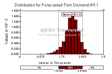
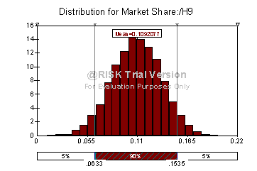
For price, we used a mean input of $378 with a standard deviation of $6; for advertising, we used a mean of $93,325 with a standard deviation of $9,828. For both variables, we assumed a normal distribution given the earlier results of our data analysis. The corresponding outputs are: market share of 10.92% and demand of 2,158 units . It is evident from this analysis that the mode average price and average advertising are the most likely values for next quarters’ input estimates since they occurred most frequently during our simulation. Using this information, we can plan production schedules for 2,034 units, giving us a market share of 10.36%. This outcome is not certain and is subject to change. Therefore, we should develop contingency plans for both the best and worst case scenarios. In the best case scenario, we would be required to increase production to meet the demand of 3,160 units, increasing our market share to 20.71%. In the worst-case scenario, we would be required to scale production down to 339 units, drastically reducing our market share to 1.08%. By examining these inputs, we can see the best and worst-case scenarios are not likely and that the industry average price will probably fall between $368 and $388. Likewise, the average industry advertising expenditures for the next quarter will most likely be between $77,151 and $109, 486. From this information, we can determine our pricing and advertising strategies for the upcoming quarter.

Through Monte-Carlo simulation, we can predict with 90% probability that the range for our firm’s demand will be between 1,616 and 2,611 units.

This demand range will result in market share between 6.33% and 15.35% for our firm in the whole industry.

Conclusion:

The knowledge of the most probable demand range is useful so that we can plan production and manufacturing activities more accurately, thereby increasing our efficiency and minimizing costs. Monte-Carlo simulation has also enabled us to better gauge the risk associated with our pricing and advertising decisions compared to the industry norms so as to maximize profits.