
Essential Regression and Essential Experimental Design are compiled Microsoft ExcelÒ Macros (Add-ins). In other words, Microsoft Excel is needed to run them. They were developed for Microsoft Excel Versions 95 and later. We recommend using Microsoft Excel 7.0 for Windows 95 or Excel 97 (Version 8.0). It has not been tested for versions of Excel beyond 97. We cannot guarantee it will work on newer versions. We will try and upgrade the software if necessary when later versions of Excel arrive.
Essential Experimental Design and Essential Regression come on a 3.5" disk. To install the software, run setup.exe on the disk.
Insert the disk in your diskette drive. In Windows 3.x, if the disk drive is named drive A, start the File Manager and activate the file list for drive A. You can either double-click the setup.exe file in the file list (Windows 3.x) or select File, Run, and then type "setup.exe". In Windows 95, you can either double-click the "My computer" icon, then do the same with the "3 Ẅ Floppy [A:]" icon and then double-click the "setup.exe" file, or you click on the Start button, select Run and type "a:\setup.exe".
By default, setup.exe will install the program files to "C:\eregress". You can choose a different destination if you prefer. Setup will also install a program group "Essential Regression" in the start menu (Windows 95) or the Program Manager (Windows 3.x).
Note: Setup.exe will not install the data file er_test.xls which is also on the program diskette. Please copy this file manually from the diskette to the directory in which you installed Essential Regression (C:\eregress by default).
From within MS Excel
In Excel, with at least one empty workbook open, select the File,Open menu. Locate ER22.xla in c:\eregress (or the directory you installed the program into) and open it. This will start the Add-In and, after an introductory screen, add a new Regress menu to the Excel main menu bar between the File and View menus.
From outside MS Excel
In Windows 95, select Start à Programs à Essential Regression à Essential Regression. In Windows 3.x, double-click the Essential Regression Icon in the Essential Regression Program Group.
Like any other Excel file, Essential Regression (ER22.xla) can also be opened directly in the File Manager (Windows 3.x) or Explorer (Windows 95) .
MS Excel will start up (or simply become the active application if it was started up before), and, after the introductory screens, a new Regress menu will be added to the Excel main menu bar between the File and View menus.
Note: Paragraphs in italics are meant only to point to additional features of Essential Regression. You are not supposed to execute them. However, if you do so, your screen could look different from what is given in the text and you should go back to the point before you "took the detour".
Open the Excel workbook "er_test.xls" which you should find in the Essential Regression program directory (provided you copied it from the program diskette, see chapter "Installation"). On the "data" worksheet, this workbook contains a small data set. The regressor variables X1 and X2 and the response, Y, are arranged in columns, the observations are arranged in rows. Any data table to be analyzed with Essential Regression should be arranged like this. The "A" column contains the index number of each observation. In columns "B" and "C", you’ll find the effects or x variables. Column "D" contains the response or Y variable.
Cell "B1" is highlighted in red. It is the leftmost cell in the header row of the range with useful data (not counting the index column). We call it the "pivot cell" of the data table. Please select this cell.
Note: It is important to select the pivot cell in a data table before launching Essential Regression!
In the Regress menu, select Multiple Regression. This will activate the Multiple Regression Input Dialog.
To select the response variable, click the "down arrow" in the Response (Y) drop-down list box. The list box should show the variables. Select the "Y" variable as the response.
Now focus on the two "Select Factors" windows in the dialog box. To select factors or input variables, add "X1" and "X2" from the list in the left window to the right window by using the ">" button between the windows. Do not add the response or y variable to the right window. If this happens, you can remove it using the "<" button.
Go to the "Type of Regression" drop-down box and select "Full Quadratic" from the list.
Do not change the remaining options. The dialog box should now look like this:
Click " >>Next>>". This opens the "Multiple Regression" Main Dialog.
In the upper left quadrant of the "Multiple Regression" Main Dialog you’ll find the "Select Term" window with a list of all possible terms in the model based on the "Full quadratic" model selected in the previous dialog: linear, squared, and interaction terms. Note that Essential Regression creates this list for you automatically. Using the arrow buttons, model terms can be added or deleted from the model after selecting them in the corresponding window. The terms currently in the model are listed in the "Current Model" Window. Note that any subset of the regression model selected in the previous dialog under "Type of Regression" can be created.
Select "X1" in the "Select Term" window and click the ">" button. Repeat this with "X2". This creates a linear model with these two terms. To perform the regression, click the "Regress" button to the right of the "Current Model" window. This executes the regression analysis and the dialog should now look like this:

The "Multiple Regression" Main Dialog displays most of the results needed to evaluate a regression model instantly. In the "Output" area, the "Summary", "ANOVA", and regression coefficients or "Term" window show the parameters needed to assess the quality of the selected model. For example, you can see that the coefficient of determination R2 for the linear model is .984, the adjusted R2 is .984, and the so-called R2 for prediction, estimating the prediction accuracy of the model, is .982. In the ANOVA table, the F-value is high (1432), and the F-significance is very low (3.75e-42), indicating a highly significant regression model.
What if you want to evaluate other models based on the selected variables "X1" and "X2"? How does the full quadratic model compare to the linear model ?
 Select the first term in the
"Select term" window and click the ">" button repeatedly until all
the 5 possible terms are in the model. Note that the "Output" area is cleared
when doing that. Now click on "Regress" again. The dialog should look like this:
Select the first term in the
"Select term" window and click the ">" button repeatedly until all
the 5 possible terms are in the model. Note that the "Output" area is cleared
when doing that. Now click on "Regress" again. The dialog should look like this:
These are the results for the full quadratic model. You can see that all three R2 parameters have improved. This can be checked easily by clicking the "Previous" button. The "Previous model summary" is displayed:
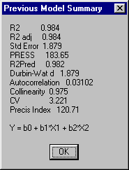
However, a look at the "ANOVA" and coefficients window shows that the F-value has decreased (from 1432 to 754), and, more obviously, some of the model terms have a low significance, i.e., the probability output for the t-statistic in the coefficients window shows numbers >0.1 (remember: the smaller the significance number in the table, the more significant the term).
Apparently, our model contains "unnecessary" terms. How can we find out fast what is the "best" model among the possible combinations of linear, quadratic, and interaction terms? In Essential Regression, we have the possibility to perform forward and backward stepwise regression based on a threshold significance which can be adjusted by the user.
You’ll find buttons for forward selection or backward elimination of model terms in the "AutoRegress" area in the upper right corner of the dialog. For example, using the full quadratic model with 5 terms, we could use the "<<Back Elim<<" button now to remove insignificant terms from the model in a stepwise fashion.
Another possibility is the use of the "Fit All" Button (can be used with no model terms selected in the Main Dialog) to get a list of all possible models (31) sorted by decreasing R2 and R2 adjusted. If you do that, you’ll get another worksheet with a list of all possible subsets of our 5 term quadratic model.
However, one of the exceptional features of Essential Regression is the "AutoFit", i.e., the automatic selection of the "best" model using repeated forward and backward stepwise regression until no further improvement can be detected.
Using the dialog as shown above as a starting point, press the "AutoFit" button in the "AutoRegress" area (upper left corner). Note that the progress is indicated in the Excel status bar at the bottom of the screen. After a few seconds, you should get the following message:

Click "OK", and the dialog should look like this:

The selected model contains the terms "X1", "X2", "X1*X1", and the constant term or intercept. Note that this model does not generally have higher R2 terms than the full quadratic model (the R2 for prediction is only slightly higher), but the F-value is higher (1284) (or, meaning the same, the "F-Significance" value is lower), indicating a more significant model. All the model terms are highly significant, indicated by the very low "Significance" values in the coefficients window.
If you execute the "Fit All" option described further above, you’ll see that the model the "AutoFit" came up with is actually not the best model available in terms of the R2-values. However, the 3 "better" models all have insignificant, i.e., redundant terms!
The "Multiple Regression" dialog allows to perform model adequacy checking. The "outlier" button produces a list showing outliers , leverage, and influential cases in our database. The "Graph" button opens another dialog which shows a variety of scatter plots useful for residual analysis.
For example, click the "Graph" button and then "Add Trendline" in the graph dialog. It should look like this:

This graph shows a plot of the y-values predicted by the model ("Y predicted") vs. the observed "Y" values and the corresponding linear trend line. As you can see, a variety of plots is available which can be selected with the arrow buttons.
So far we only could see the results of the regression analysis in dialog boxes. Now, we will create a permanent Excel output worksheet. Exit the graph dialog shown above and press the "Make XLS" button in the main dialog. After a few seconds, the following message should appear. Click "OK" and then "Exit" in the main dialog.

After exiting the main dialog, the output sheet ("data_1") should be the active window.
Note the buttons on the left hand side in the first column. By pressing these buttons, you can perform a series of useful actions:
-Reregress the model (goes back to the Main Dialog),
-Delete the output sheet if needed,
-Predict new responses based on new data points,
-see scatter plots similar to the ones described above for residual analysis ("Graph"),
-evaluate a data table including residual analysis for each data point,
-go to a regression coefficients table like the one in the main dialog,
-"optimize", i.e., find a set of inputs which gives a specific output,
-check the confidence ranges for the regression in a scatter plot,
-view the outlier table,
-print selected output ranges from the sheet,
-look at the correlation matrix (R matrix).
Finally, the "surface" button allows you to see a 3D surface of you regression model equation, provided there is more than one variable in your model.
In our example, the equation we arrived at after using "AutoFit" contained "X1" and "X2" (as the squared term). On the output Excel sheet you just created, press the "Surfaces" button. In the next message box, click "OK":

The next dialog shows a list of the available variables to plot. In our case, there is only one 3D plot possible: the reponse ("Y") vs. "X1" and "X2".
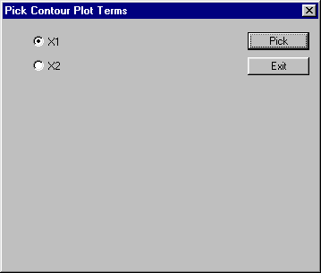
Select "X1" and click the "Pick" button. In the next message box, click "OK".
Select "X2", and click the "Pick" button again. Essential Regression creates the surface plot, and you should see the following graph on your worksheet:

If you click the "Contour" button above the graph, you get the 2D representation of the surface, a contour plot. The "Contour" button changes to a "3d" button. Pressing it brings back a surface plot.
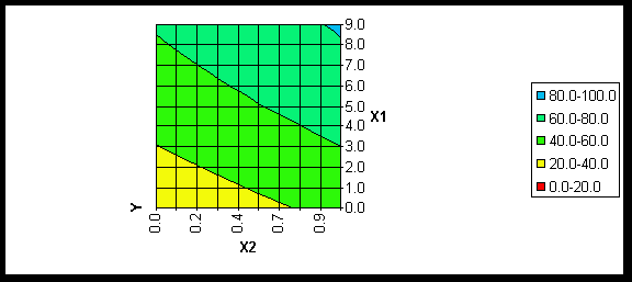
You can rotate the graphs by using the "<" and ">" keys. Also, you can increase or decrease the number of levels by clicking "+" or "-", respectively. In our example, we have used the "+" key a few times to bring out more colors.
If your model has more than 2 variables, you will find another button above the graph area with the caption "movie". The "movie" feature allows you to incrementally change the value of one variable while plotting the response vs. two other variables. If you loop through these changes, the effect resembles an animation or movie with the surface changing according to the value of the changed variable.
Pressing the "Back" button at any time takes you back to the starting point, i.e., the upper left corner of the worksheet.
Make sure that you save the Excel worksheet before closing Excel if you wish to keep the output. Basically, this sheet generated by Essential Regression (ER) is a standard Excel worksheet linked to ER through the added buttons.
This tutorial is intended to lead you through a relatively simple regression analysis while emphasizing the features of Essential Regression which allow for a quick assessment of the model. There are many more features explained in detail in the previous chapters.
In Excel simply select the Regress, Unload menu option this will close Essential Regression and remove the Regress menu from Excel.
From within MS Excel
In Excel, with at least one empty workbook open, select the File, Open menu. Locate EED22.xla in c:\eregress (or the directory you installed the program into) and open it. This will start the Add-in and, after an introductory screen, add a new DOE menu to the Excel main menu bar between the File and View menus.
From outside MS Excel
In Windows 95, select Start, Programsà Essential Regression à Essential Experimental Design. In Windows 3.x, double-click the Essential Experimental Design Icon in the Essential Regression Program Group.
Like any other Excel file, Essential Experimental Design (EED22.xla) can also be opened directly in the File Manager (Windows 3.x) or Explorer (Windows 95) .
MS Excel will start up (or simply become the active application if it was started up before), and, after the introductory screens, a new DOE menu will be added to the Excel main menu bar between the File and View menus.
We assume EED is loaded and the DOE menu is visible. First, select the Design An Experiment option in the DOE menu. This brings up the Design an Experiment Dialog. We are going to create a circumscribed central composite design (CCD) with 3 factors and 4 center points to assess curvature and experimental error. Please make the appropriate selections. The dialog should look like this before you continue:

In the colored section at the bottom, the dialog shows that our design has 18 runs or experiments (including the center points), and that the underlying model has quadratic terms.
Press the "Make DOE" button. EED creates the "Aliasing" worksheets giving information how certain effects are aliased with others, and the Factor Definition Dialog will be displayed:
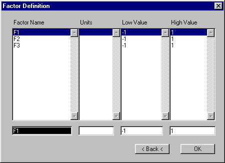
Here, you can set the lows and highs for the design factors. For our purposes, simply accept -1 and 1 as low and high settings for the design and continue with "OK". EED will create the "Experiments" worksheet and the following confirmation message will appear. Simply press "OK" to continue:

In the "Experiments" worksheet, you’ll find information about your design and the underlying model. Let us pretend we would conduct the 18 experiments necessary to analyze the model. In EED, we can simulate this process. In the DOE menu, select Simulate Data. This will bring up the Data Simulation Input Dialog. Accept "Resp_1" as the response name and select the Factors F1, F2, and F3 as the model factors. Further, let’s assume we have a linear model (you can change the model type in the "Type of Model" list box at the bottom of the dialog). The dialog should now look like this:

Press the ">>Next>>" button. This will bring up the Input Model Coefficients Dialog. Select "F1" (factor 1) in the window listing the "Possible Model Terms". Then type the value for the coefficient for factor 1 into the edit box shown below the "Initial Coefficients" window. The cursor should be activated in this edit box by default so that, after selecting "F1", you should be able to type directly. Enter "5" as the value for the coefficient.
Repeat these steps for the factors F2 and F3 using "10" and "-15" as coefficients. After that, enter "10" as a value for the constant term in the model and leave the noise standard deviation at 1. The dialog should then look like this:

This concludes the model definition. What we have done is to simulate a linear regression model as the basis for our experimental design. Press the "Make Data" button, and EED will calculate "responses" for each experiment on the "Experiments" worksheet. Note that the data table now contains data in the response column.
Let’s pretend we do not know the exact model equation which we just have used to calculate our data. The next step will be a multiple regression to come up with a model which describes our data best.
To perform this task, select Analyze Design in the DOE menu (the "Experiments" worksheet should be the active sheet when doing this). This will launch Essential Regression in "EED mode", and a Multiple Regression Input Dialog different from the one shown in Chapter 7.4 will come up:

By default, this dialog selects "Resp_1" as the column of the data table containing the response. Accept the defaults and click ">>Next>>". This will bring up the Multiple Regression Main Dialog (see Chapter 7.4). At this point, simply click the "AutoFit" button and have Essential Regression find the best model. The outcome depends on the data you simulated as described previously. The random error or noise term we introduced can lead to different results as far as the optimized model is concerned. However, the model you end up with should contain F1, F2, and F3 as highly significant factors and possibly another, higher order term with less significance.
You could click the "Fit all" button in the Multiple Regression Main Dialog and find out which model is the "best", based on R2 and R2 adjusted. If you limit the number of factors to 4, this should not take unreasonably long.
Also, note that you are now in Essential Regression (ER). You can use all the features of ER including 3D- graphing. Since you have 3 variables, you can use the "movie" feature in the surface plot area of the output sheet (described in chapter 7.4).
In Excel simply select the DOE, Unload menu option this will close Essential Experimental Design and remove the DOE menu from Excel.
This book was meant as a supplement to the Essential Regression and Essential Experimental Design Add-Ins. We put in as much information about Linear Regression and DOE as we thought was reasonable to enable any user of this software to perform a meaningful analysis. We are aware that,by doing so, we had to cut corners here and there and sometimes even leave out topics which, in the eyes of a really serious reader (or a statistician), should have been discussed.
For people interested in the fundamentals and the mathematical details, we recommend studying some of the following publications. We, not being statisticians by trade, necessarily had to distill much of the information presented in these literature references into this book and, hopefully did not make too many mistakes in doing so. We think everybody applying statistics on a regular basis should peruse some of the books listed below:
Douglas C. Montgomery and Elizabeth A. Peck, "Introduction to Linear Regression Analysis", 2nd Ed. 1992, John Wiley & Sons, Inc., New York, NY (ISBN 0-471-53387-4).
Raymond H. Myers, Douglas C. Montgomery, "Response Surface Methodology, 1995, John Wiley & Sons, Inc., New York, NY (ISBN 0-471-58100-3).
Douglas C. Montgomery, "Design and Analysis of Experiments", 3rd Ed., 1991, John Wiley & Sons, ew York, NY (ISBN 0-471-52000-4).
Lyman Ott, "An Introduction to Statistical Methods and Data Analysis", 3rd Ed. 1988, PWS-Kent Publishing Co. Boston, MA (ISBN 0-534-91926-X).
Jay L. Devore, "Probability and Statistics for Engineers and the Sciences", 3rd Ed. 1991, Brooks/Cole Publishing Co., Pacific Grove, CA (ISBN 0-534-14352-0)
For readers interested in the details of nonlinear regression analysis:
Douglas M. Bates, Donald G. Watts, Nonlinear Regression Analysis ad its Applications, John Wiley & Sons, Inc., New York, NY (ISBN 0-471-81643-4).