http://www.oocities.org/SiliconValley/Peaks/8778/TAU_advprog.html
5 Trees
5.1 Examples of trees.
There are many situations when information has a hierarchical or
nested nature. Well known examples of this are: family tree or
organization chart. The abstraction of such structure is called
a "tree" and this data model is one of the most fundamental data
models. BTW, you are using such a tree all the time you are working
on a computer: most of modern operating systems have file system
organized as a tree:
dir1
|---dir2
|   |---file1
|   |---file2
|   |---dir3
|---dir4
    |---file3
5.2 Advantages of trees
Why are trees so useful and frequently used? Because they have some
very serious advantages:
- "unlimited" size (like a linked lists)
- fast insertion/search by key
- possibility to create hierarchical data structure
- still easy to implement
5.3 Formal definition of trees
An abstract tree is a set of points, called "nodes", and lines
called "edges". An edge connects 2 distinct nodes. To be a tree
such a set must satisfy the following properties:
- There is one "special" node in a tree, it is called the "root".
- Every other node (not root) "C" is connected (by an edge) to
some one other node "P". This node "P" is called the "parent" of "C",
and "C" is called a "child" of "P".
- All nodes are connected to the root (of course, via their parents).
So we have already 3 terms: "root", "parent" and "child". Let's define
some more:
- A parent of a node, a parent of the parent and so on are
called "ancestors" of the node. (Strictly speaking a node is also
its own ancestor.)
- A child of a node, a child of the child and so on are called
"descendants" of the node.
- If m1, m2, ..., mk are such
nodes that m1 is the parent of m2, m2
is the parent of m3, ..., mk-1 is the parent
of mk then m1, m2, ..., mk
is called a "path" from m1 to mk in the
tree. The "length" of this path is k-1, i.e. this is a number of the
edges we have to "pass" going this path. (Again, strictly speaking
one node is also a path with zero length.)
- If length of a path between 2 nodes is more than 0 than the upper
node is called a "proper ancestor" and the lower node is called
"proper descendant".
- Nodes that have the same parent are called "siblings".
- The length of the longest path from a node to its descendant
is "height" of the node.
- Height of the root is called "height of the tree".
- The length of the from the root to a node is "depth" or "level"
of the node.
Well, now we have more terms: "ancestor", "descendant", "path in
tree", " proper ancestor", "proper descendant", "sibling", "height
of node", "height of tree" and "level of node".
There are more terms used for, for example, trees where all child
of the same parent have their own order, etc. We will define them
when and if we will need them.
5.4 Operations on trees
Let's see which operations on trees may be defined:
- search
- insertion of node
- deletion of node
- deletion of subtree
- merge of 2 trees
- traversing tree
- etc. etc. etc.
5.5 Various types of trees and tree implementations
There are many types of trees and, correspondingly, there are many
ways to represent a tree. Anyway two of the possible representations
are the most usable. These are:
- Common trees. These are representations of a tree when each
node has unlimited possible number of children. Such trees are
usually implemented as "list of lists", namely in one of 2 ways:
- Array-of-Pointers, when each node has an array of pointers
looking to its children;
- Leftmost-Child-Right-Sibling, when each node has 2 pointers:
one - to the leftmost child of it and another one - to the next
right child in its sibling.
- Binary trees. This is a special case of trees which can satisfy
many tasks where a tree is needed. Binary tree is a tree where each
node can have not more than 2 children. The words "binary tree" have
a shortcut "B-tree".
5.6 Binary trees
The most usual case when a B-tree is used is storage of ordered
information. In this case we can store all elements, say, "more
or equal" then element in a node in one subtree of this node while
all elements "less" than this are stored in the second subtree.
Let's take for our further discussion B-tree that will store unique
integer numbers (i.e. each number will be stored in the tree only
once). In this case we can define a node of the tree so:
typedef struct tree_node
{
	int val;
	struct tree_node* gt;
	struct tree_node* lt;
} TNODE;
So the "gt" will point to subtree where all values are greater of
"val" of the node and "lt" will point to subtree where all values
are less then "val".
Use of structures like that allows us to easily write many algorithms
in recursive way:
{
	action A0;
	recursive call on left subtree;
	action A1;
	recursive call on right subtree;
	action A2;
}
Let's look how we can do it for our B-tree of integers. The simplest
example is a printing of the tree:
void print_tree( TNODE* tree)
{
	if( tree == NULL)
		return;
	print_tree( tree->lt);
	printf( "[%d] ", tree->val);
	print_tree( tree->lt);
}
5.6.1 Search in B-tree
This is a function checking if the tree contains an integer:
int lookup( TNODE* tree, int v)
{
	if( tree == NULL)
		return( 0);
	if( v == tree->val)
		return( 1);
	if( v < tree->val)
		return( lookup( tree->lt, v));
	else
		return( lookup( tree->gt, v));
}
The running time of this algorithm is dependent on the tree
organization: it may vary from O(log2N) (in the best
case) to O(N) (in the worst case). We will see why in the insertion
algorithm.
Just to compare we can write this function in iterative manner too:
int lookup( TNODE* tree, int v)
{
	TNODE* n;
	for( n = tree; n != NULL; )
	{
		if( n->val == v)
			return( 1);
		if( n->val < v)
			n = n->lt;
		else
			n = n->gt;
	}
	return( 0);
}
Well, for the "lookup" function the difference looks not so
significant but for more complicated algorithms (e.g. deletion from
the tree) it is really painful to write an iterative function.
5.6.2 Insertion of a node to B-tree
The insertion to a binary thee is a pretty simple work:
TNODE* insert( TNODE* tree, int v)
{
	if( tree == NULL)
	{

		tree = (TNODE*)malloc( sizeof( TNODE));
		tree->val = v;
		tree->gt = tree->lt = NULL;
	}
	else if( tree->val > v)
		tree->lt = insert( tree->lt, v);
	else if( tree->val < v)
		tree->gt = insert( tree->gt, v);
	return( tree);
}
Please not that in case when numbers are inserted in order of their
increasing of decreasing our tree will degenerate to a simple singly
linked list. So in this really worst case the running time if the
algorithm becomes O(N). In the best case when all numbers are really
random we can expect that each node will have approximately 2 children,
so the running time will be O(log2N). We will discuss how
to avoid such situation a little bit later (in balanced trees).
5.6.3 Deletion of a node from B-tree
Deleting an element from a B-tree is a little bit more complicate
than "lookup" or "insert". If the node to be deleted is a leaf then
it must be simply deleted. The problem arises when the node is
interior. Then we can not delete it due to this will causes
disconnecting the tree. So we must rearrange the tree in a way
preserving our "greater " and "less" relationships between
nodes. Let's distinguish 2 cases. First, if the node has only 1 child
then we can replace it by that child, and everything will be
OK. Second, if there are both children. One of possible strategies is
to find the node "m" with the smallest element in the "greater"
subtree of our node, and replace our node by the node "m". So, let's
write a function that will find the node with the minimal element
for some node (in other words: to find the descendant with the
minimal value):
TNODE* detach_min( TNODE* node, TNODE* prev0)
{
/* this function is called only if "node" has "less" children */
	TNODE* n;
	TNODE* prev = prev0;

	for( n = node; n->lt != NULL; n = n->lt)
		prev = n;
	/* now we found the node with the smallest element - "n" */
	/* and "prev" is its father */

	/* well, now n has no "lt" child, so we can force "prev" */
	/* to "forget" about it */

	/* let's handle a special case when we have reached */
	/* the minimal node immediately, i.e. it is the "gt" */
	/* child of our node */
	if( prev == prev0)
		prev->gt = NULL;
	else
		prev->lt = n->gt;

	return( n);
}
Now let's write the main "deletion" function:
TNODE* remove_node( TNODE* tree, int v)
{
	TNODE* tmp;
	if( tree == NULL)
		return( NULL);
	if( tree->val > v)
		tree->lt = remove_node( tree->lt, v);
	else if( tree->val < v)
		tree->gt = remove_node( tree->gt, v);
	else /* OK, "tree" is the node to be deleted */
	{
		if( tree->gt == NULL)
		{
			tmp = tree;
			tree = tree->lt;
			free( tmp);
		}
		else if( tree->lt == NULL)
		{
			tmp = tree;
			tree = tree->gt;
			free( tmp);
		}
		else	/* the case of both children presented */
		{
			tmp = detach_min( tree->gt, tree);
			tmp->gt = tree->gt;
			tmp->lt = tree->lt;
			free( tree);
			tree = tmp;
		}
	}
	return( tree);
}
By the way, here you can see an example when in one case iterative
function fits our needs better (at least looks simpler, and therefore,
understandable) while in another case recursive function is much
more clear.
5.6.4 Balanced trees. AVL trees
5.6.4.1 Disadvantages of simple B-trees. The main idea of balanced
trees.
As we saw there is a possibility to get a degenerate B-tree in case
of ordered insertion, i.e. instead of tree we have a simple linked
list. It was obvious from the very beginning and people tried to
solve this problem in various manners. The general purpose of all
such methods was to keep the tree as balanced as possible all the
time. "Balanced" means that number of the "left" descendants must
be as close as possible to number of the "right" descendants of each
node in the tree. It is clear that such a improvement of the regular
B-tree should be in the "insert" operation only.
One of the most "trivial" ideas is to keep track of the root's "left"
and "right" subtree heights and to completely reorganize the tree
when the difference exceeds some constant. Unfortunately such a
periodical reorganization of a tree also beats the running time of
the insertion algorithm.
5.6.4.2 The
main idea of the AVL algorithm.
One of the best solutions (used up today) was suggested by 2 people:
Adelson-Velsky and Landis in 1962. This solution got its name from
their last names and is called AVL-trees.
Let's look what's going on when we are inserting a new node. In fact
we have only 2 situations breaking the balance:

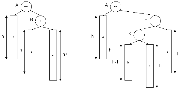
(This picture shows possibilities of unbalancing after insertion
of value going to right subtree of A. Two more cases are identical if
we reflect these diagrams, interchanging left and right). Case 1
occurs when a new element has just increased the height of node B's
right subtree from h to h+1. Case 2 occurs when the new element has
increased the height of B's left subtree.
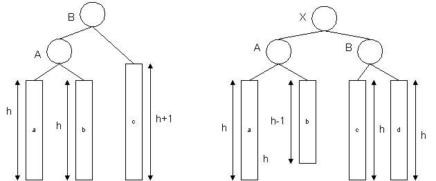
We can perform simple transformations to keep the tree balanced for
the both cases. In Case 1 we simply "rotate" the tree to left,
attaching "b" to A instead of B and B becomes to be root. In Case 2
we use a "double rotation", first rotating nodes (X,B) right, then
nodes (A,X) left, so X becomes to be root.

The number of operation for both types of rotations is a constant, so
the AVL-tree keeps the running time of the insertion O(logN) all the
time.
5.8 Not binary trees
Binary trees are only one (although very commonplace) case of
trees. Let's see how "more common" (meaning trees where a node can
have more than 2 children) trees can be implemented.
5.8.1 Children vector (Array-of-Pointers)
This is one of the simplest ways to represent a tree: each node is
a structure consisting of both some node-specific information and
an array os pointers to the children of the node. The size of that
array of pointers is the maximum number of children a node can have,
this number is called "branching factor". If some element of the
array does not point to a child then it has value NULL.
This representation allows us to access any i-th child of a node very
quickly. However this representation is very memory-consuming if
only few nodes in the tree have many children - then most of our
pointers will be NULL.
5.8.2 Trie
There is one particular case of "Array-of-Pointers" trees, that have
its own name: "TRIE". (This word came from the word "reTRIEve". It
is pronounced now like "try" not "tree" to distinguish tries from
other trees.)
What is a trie? Let's look an example. Suppose we want to store a
collection of words in a way that makes it quite efficient to check
the presence of a word (i.e. sequence of characters) in this
collection. Well, let's build a tree where each node (excepting the
root) has an associated letter. The string of characters representing
by a node is the sequence of letters along the path from the root to
this node. The information on a node consists of the letter
(represented by the node) and some sign telling whether the path from
the root to this node is a complete word.
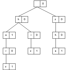
For instance, suppose we have a "dictionary" with the following
words:
A trie for these words may be such:

So the word "him" will be not fount in the trie, while all "our"
words will be found. Also the word "her" will not be found in the
trie as a complete word.
Well, we can use the following structure to represend such a trie
(assuming that our dictionary is case-insensitive):
typedef struct trie_node
{
	char			letter;
	int			end_of_word;
	struct trie_node*	children[26]; /* 0 - a, 1 - b, ... */
} NODE;
Do not think that such tries are useful for dictionaries of "real"
words. The same approach may be used when we need store other
sequences of "elementary" creatures: e.g. phone numbers or ID numbers
are "words" of digits where common subsequences are often, more
complicated example: structures of compounds in organic chemistry are
very frequently chains of some simpler compounds or components, so
a dictionary of organic compounds may be built with a trie also.
5.8.3 Sibling
A more full name of this type of tree representation is
"Leftmost-Child-Right-Sibling".
typedef struct LCRS_node
{
	int			val;
	struct LCRS_node*	leftmostChild;
	struct LCRS_node*	rightSibling;
} LCRS_NODE;
Function lookup() may look so:
int lookup( LCRS_NODE* tree, int v)
{
	if( tree == NULL)
		return( 0);
	if( tree->val == v)
		return( 1);
	if( lookup( tree->leftmostChild, v))
		return( 1);
	return( lookup( tree->rightSibling, v));
}
5.9 Traversing tree
There always are operations you want to perform on each node of a
tree. Such a traversing may be easily implemented by recursive
operations on the tree that can be written naturally and
cleanly. Generally speaking if we have a node n that has k children
(c1,...,ck) then we can write such a function
in the following manner:
F(n)
{
	action A0;
	F( c1);
	action A1;
	F( c2);
	action A2;
	...
	F( ck);
	action Ak;
}
There are some more often used types of traversal functions.
5.9.1 Preorder
The main form of a preorder traversal function is:
{
	action on the node;
	recursive call on subtrees;
}
So the action on the node is performed BEFORE its children. For
example, printing of our Leftmost-Child-Right-Sibling tree of integers
may look so:
void preorder_print( LCRS_NODE* tree)
{
	LCRS_NODE* n;

	if( tree == NULL)
		return;
	/* our action - to print the value */
	printf( "%d\n", tree->val);
	/* now the same for all children */
	for( n = tree->leftmostChild; n != NULL; n = n->rightSibling)
		preorder_print( n);
}
5.9.2 Postorder
Unlike the preorder traversing here we perform our action on a node
AFTER visiting the node's children:
{
	recursive call on subtrees;
	action on the node;
}
And our printing of the tree may look so:
void postorder_print( LCRS_NODE* tree)
{
	LCRS_NODE* n;

	if( tree == NULL)
		return;
	/* first the same for all children */
	for( n = tree->leftmostChild; n != NULL; n = n->rightSibling)
		postorder_print( n);
	/* our action (to print the value) - after passing children */
	printf( "%d\n", tree->val);
}
5.9.3 Inorder
Mainly the inorder traversing makes sense for binary trees. In general
it looks so:
{
	recursive call on left subtree;
	action on the node;
	recursive call on right subtree;
}
Examples of inorder traversal functions was given before - in fact
almost all the functions we had for binary trees were built in this
manner.
For not-binary trees we also can use the inorder traversing in case
when we can define some relationship between nodes so, that for any
pair of nodes we can say which one "goes first" (or which node is
"less" or which one is "greater"). In this case we can go first to
all children "less" the current node (in order of their "growing"),
then perform our action on the node itself, and then to go to all
"greater" children.
5.10 Important tree applications
5.10.1 Expression trees
In many applications it is necessary to parse and evaluate some
expressions. e.g. arithmetical expressions. The most handy way to do
this is to represent an expression in some tree. For example, if we
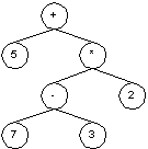
have an expression:
5 + ( 7 - 3) * 2
then it can be easily stored in some tree where leafs represents the numbers and interior nodes represents the operations:

A function to evaluate (to find the result) for such trees will look
somehow so:
int eval( NODE* tree)
{
	if( no children)
		return( tree->val);
	switch( tree->operation)
	{
	case OP_PLUS:
		return( eval( tree->left) + eval( tree->right));
	case OP_MINUS:
		return( eval( tree->left) - eval( tree->right));
	case OP_MULTIPLY:
		return( eval( tree->left) * eval( tree->right));
	case OP_DIVIDE:
		return( eval( tree->left) / eval( tree->right));
	}
}
5.10.2 Syntax trees (Parse trees)
Syntax trees is a kind of trees very similar to the expression
trees. If we take some formal language (like most programming
language, e.g. C) then the structure of the entire program may be
represented as a sequence of some constructions (in case of C - new
types definitions, external variable declarations and functions). Each
of these constructions is in turn also some sequence of other
subconstructions, and so on. So we can represent the entire program
as a tree where leafs will be some elementary lexems, like numbers,
keywords, etc. On other hand, we can describe the syntax of such a
language as a tree where each node (construction) contains children
that are possible (for this particular construction)
subconstructions. So the whole definition of some formal language may
be represented as a tree - such a representation makes much easier
the task of parsing of a text written in this language.
It is very complicated task to build such trees for not formal
languages like people languages (e.g. English, Hebrew) or mathematical
prove language (where formal mathematical symbols appears with free
text) etc. Nevertheless even in such cases the most matching approach
to analyze them is to use some more "smart" and flexible syntax trees.
5.10.3 Decision making trees
In fact any program is a tree of actions:
if(some condition)
	do something
else
	do something else
etc.
But if a program should work for very big and often changing set
of conditions then it becomes very complicated (if possible at all)
task to write such a program. Trees can greatly help here also: if
we represent each condition as an interior node and actions as leafs,
then we can handle it - it will be enough to go from root through
all conditions we have to check (eliminating not needed checks
remaining in other branches of the tree) while we reach some
leaf - this is the action we have to perform. Moreover such
representation is very flexible: if the set of our condition changed
somehow the only thing we have to do is to rebuild our tree - and
the program is ready to work again. Such trees are called "decision
making trees".
