http://www.oocities.org/SiliconValley/Peaks/8778/TAU_advprog.html
6 Graphs
Generally speaking, a graph is a data model just to work with a
binary relation. However it has a powerful visualization as a set
of points (nodes) connected by lines (edges) or by arrows (arcs). So
the trees discussed above are a particular case of graphs.
6.1 Examples of graphs
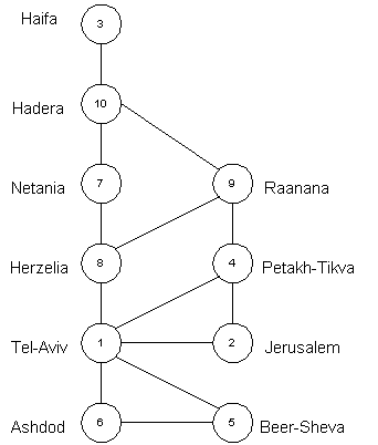
Let's take several cities connected by roads.

This is a graph representing connectivity of the cities. Graphs may
be different: undirected and directed, weighted, etc. For example,
if we take some country resided on islands (e.g. Hawaiian Islands
or even Great Britain or Japan) then we get such a graph consisting
of several parts (each part will represent roads of 1 island but
there is often no road connection between islands), so we get not
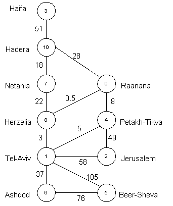
connected graph. Another example: if we want to know not only the
fact of connectivity between cities but also distances between them
then we get weighted graph:

6.2 Formal graph definition. Kinds of graphs
Let's define some basic types of graphs and terms to manipulate with
them.
A "directed graph" consists of:
- A set of N "nodes".
- A binary relation A on N. A is called set of "arcs" of the
directed graph.
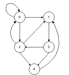
For example:

The set of arcs for this graph is:
A = { (0,0), (0,1), (0,2), (1,3), (2,0), (2,1), (2,4), (3,2), (3,4),
(4,1) }
(It is written often u -> v for arc (u,v).)
For any arc (u,v) (or u -> v) v is the "head" and "u is the
"tail" of the arc.
Also u is called a "predecessor" of v, and "v" is called "successor"
of u.
If the head and tail of an arc is the same node then such an arc is
called "loop".
As for trees, where we had some arbitrary information on each node,
we can do the same for nodes of a graph. Such an attached info is
called "label". Please note: we must distinguish all the nodes in
a graph, so each node has some unique "name", while two or more nodes
can have the same label.
A "path" in a directed graph is a list of nodes (v1,
v2, ..., vk) such that there is an arc from
each node from the list to the next, i.e. there is
vi -> vi+1 for I = 1,2,...,k-1. The
"length of the path" is k-1. (Note: any node v is a path of zero
length from v to v, BUT if there is an arc (v,v) then there is also
another path with length 1.)
A "cycle" in a directed graph is a path of length 1 or more that
begins and ends at the same node. A "length of the cycle" is the
length of the path. For our example we have cycles: (0,0), (0,2,0),
(1,3,4,1), (1,3,2,4,1), etc.
A cycle can be written to start and end at any of its nodes. All
such cycles are called "equivalent cycles".
A cycle (v1, v2, ..., vk,
v1) is a "simple cycle" if only node v1
appears more than once there. For our example the cycle (0,2,0) is
simple but the cycle (0,2,1,3,2,0) is not simple. It is clear that
if there is a cycle in a graph then there must be at least one
simple cycle.
If a graph has 1 or more cycles then the graph is called a "cyclic
graph". Similarly if there is no cycles, the graph is called an
"acyclic graph".
Let's repeat the terms we has defined for directed graphs:
- directed graph
- node
- arc
- head of arc
- tail of arc
- loop
- predecessor of node
- successor of node
- name of node
- label of node
- path
- length of path
- cycle
- simple cycle
- equivalent cycles
- cyclic graph
- acyclic graph
It is useful sometimes to connect nodes by lines that do not have
directions. Such lines are called "edges", and such graphs are
called "undirected graphs". The edge {u,v} says that nodes u and v
are connected (in both directions). (Note that an edge {u,u} does
not make sense, so most books on graphs do not allow such edges
at all.)
The definition of a "path" for undirected graph is the same as for
directed one. The only thing to be noted is that edge {u,v} is the
same as edge {v,u} unlike arcs in a directed graph.
We can not define a cycle like it was for directed graphs due to
any edge is bi-directional. So let's start from the definition of
a simple cycle: a "simple cycle" is a path of length 3 or more that
begins and ends at the same node and all other nodes appear there
only once. A non-simple cycle is concatenation of 1 or more simple
cycles, but this thing is likely useless, so we will not use it.
Two undirected cycles are "equivalent cycles" if they consist of
the same nodes either in the same orders of in reverse order.
Now we have for undirected graphs the same terms as for directed
graphs excepting "edges" that are used instead of "arcs".
6.3 Graph implementations
Before we discuss various operations on graphs let's see how a graph
can be implemented. There are 2 standard ways to represent a
graph. The first way is more or less similar to what we had before
- here we store a graph using lists. The second way is something new
- there we will use matrixes.
6.3.1 Adjacency lists
The main idea here is to store for each node a list of its
successors. The list may be implemented as either an array or a
linked list or however else - depending on the needs for each
particular case. (The graph itself is also a list of nodes.) For
our example we will have the following picture of lists:
0 -> 0, 1, 2
1 -> 3
2 -> 0, 1, 4
3 -> 2, 4
4 -> 1
Please note that the list of successors must not contain the nodes
themselves but references to them (by pointers or other node
names). So the list of nodes must be stored separately from the
lists of connections.
6.3.2 Adjacency matrices
Another approach is to store the information about connections in
a matrix: if there is an arc u -> v then we will set
matrix[u][v] = 1 otherwise 0. So for our example we will have the
following matrix:
 | 0 1 2 3 4
------------
0| 1 1 1 0 0
1| 0 0 0 1 0
2| 1 1 0 0 1
3| 0 0 1 0 1
4| 0 1 0 0 0
It is clear that here we also must store separately the information
on nodes and information about the connections.
6.3.3 Comparison of the implementations
It's a little bit problematic to compare the 2 approaches in the
graph representation as the advantages and/or disadvantages of each
of them is dependent on how we use the graph. The only things that
are right always are:
- check of existence of a arc/edge is more effective on the
matrix then on the lists
- sometimes the matrix may contain not only "sign" of a connection
existence but some useful information also (e.g. for our graph of
roads we can put 0 if there is no road between cities or distance
between them - so it will be both the sign of the presence of the
road and a useful value).
For other actions on graphs we will distinguish sparse graphs (where
the number of arcs/edges is comparable to the number of nodes) and
dense graphs (where the number of arcs/edges is much greater then
the number of nodes).
So if we have a sparse graph then:
- the matrix wastes more memory then the lists
- the lists are more efficient to find successors of a node
If we have a dense graph then:
- the matrix is more efficient to find predecessors of a node
- the lists waste more memory (due to necessity to store some
technical things for the managing of the lists)
And so on. In fact, when you have to choose how to implement some
graph, you have to think first which operations you will use on it
and then make the decision.
6.4 Operations on graphs
As the 1st example let's take finding of connected components (i.e. to
finds the parts of a graph that have no connections between them). The
algorithm is quite simple. Firstly let's take all the nodes of the
graph without any arcs. So we have each node as a separate connected
component. Now we take the 1st arc in the graph and merge 2 nodes
connected by this arc to one connected component. Then we take the
2nd arc and merge 2 components connected by this arc to one
component. And so on. When we have considered all arcs/edges in this
manner, we have all the connected components of the full graph. It is
possible to prove that the running time of this algorithm is
O(m * log n) (m - number of arcs, n - number of nodes). This is not
the best algorithm. A better algorithm may be built using graph
traversing methods. Moreover the most of algorithms for graphs are
based on graph traversing.
6.4.1 Graph traversing
There are 2 ways to traverse a graph. They are called:
- breadth first search
- depth first search
6.4.1.1 Breadth first search and traversal
In breadth first search we start at a node v and mark it as having
been reached. We say that a node has been explored when we has visited
all nodes adjacent from it. All unvisited nodes adjacent from v are
visited next. These are new unexplored nodes. The first node on this
list is the next to be explored. Exploration continues until no
unexplored node is left. So the list of unexplored nodes operates as
a queue. Let's write this function in pseudocode (not in C):
BFS( int v) /* BFS stands for "breadth first search" */
{
	Queue q(SIZE);
	int u = v;
	visited[v] = 1;
	do
	{
		/* here is the place where we will be with */
		/* each node of the graph as u */
		for all nodes w adjacent from u
		{
			if( visited[w] == 0)
			{
				q.put(w); /* add to the queue */
				visited[w] = 1;
			}
		}
		if( q.empty()) /* no more unexplored nodes */
			return;
		u = q.get(); /* get the 1st unexplored node */
	} while( 1);
}
The BFS() function visits all nodes reachable from the node v. If
we are not sure that our graph is connected then we have to write
a function more to ensure visiting of all nodes:
BFT( int SIZE) /* BFT stands for "breadth first traversal" */
{
	int n;
	boolean visited[SIZE];
	/* first we mark everything as not visited */
	for( n=1; n<=SIZE; n++)
		visited[n] = 0;
	/* and to use the BFS() for not visited nodes */
	for( n=1; n<=SIZE; n++)
		if( !visited[n])
			BFS(n);
}
Please pay attention that the running time of this algorithm is
dependent on graph representation: if we have a graph with n nodes
and m arcs then for adjacency matrix we have O(n2) while
for adjacency lists we have O(n+m). Nevertheless reminding that for
a full graph (where all nodes are connected to all nodes) we have
m = n2/2+n (just imagine its adjacency matrix), the
representations become the same when we deal with a dense graph.
6.4.1.2 Depth first search and traversal
Another method to traverse graph is a "depth first search". It differs
from a breadth first search in that the exploration of a node v is
suspended as soon as a new node is reached. At this time the
exploration of the new node u begins. When this new node has been
explored, the exploration of v continues. Such a procedure may be
easily written recursively (again: this is pseudocode not C):
DFS( int v) /* DFS stands for "depth first search" */
{
	visited[v] = 1;
	for all nodes w adjacent from v
	{
		if( visited[w] == 0)
			DFS( w);
	}
}
Again this function will visit all nodes reachable from node v. So
to ensure visiting of all nodes in the graph we have to write a
function DFT(), which is similar to the BFT() discussed above.
The running time here is the same as for breadth first search.
Please note that the breadth first search algorithm is based on a
queue of nodes while the depth first search algorithm is based on
a stack (this fact is hidden by implementation via recursion).
6.4.3 Applications of the graph traversing and other important algorithms on graphs
6.4.3.1 Connected components find
A problem requiring to find connected components of a graph
(or one of them - starting from some definite node) then we
already have several solutions for it: any graph traversal
algorithm (either DFS or BFS) can be used for this.
Please note that to solve this problem the graph must be treated
as undirected (even if it is directed).
Running time (as we saw) of this task will be O(n+m).
6.4.3.2 Reachability test
A natural question often appearing for directed graphs: is there
a path from node u to node v? Or in more general form: if to start
from node u then which nodes can be reached?
The simplest way to solve this problem is (like in the previous case)
to use one of the search algorithm (either DFS or BFS) discussed
above.
Naturally the running time of this task will be again O(n+m).
6.4.3.3 Topological sort for undirected acyclic graphs
Suppose we know that a directed graph is acyclic.
We want to find such list of its nodes (v1,
v2, ..., vk) that for each edge
vi -> vj the node vi goes in
the list before the node vj.
There are many examples when such a task must be solved. Let's take
one of them - a simple case of planning task: you have a list of
tasks, and you know that some tasks are dependent on completion of
some certain other tasks. If you represent tasks as nodes and the
dependencies between them as edges then after getting such a "sorted"
list of task you get the order, in which the tasks can be
performed.
The algorithm solving this problem is based on DFS(). Let's start
DFS() from some node vi and store node in a stack
in postorder manner:
DFS( int v) /* DFS stands for "depth first search" */
{
	visited[v] = 1;
	for all nodes w adjacent from v
	{
		if( visited[w] == 0)
			DFS( w);
	}
	push node v into the stack
}
After the 1st run of DFS() we got in our stack all nodes reachable
from the node vi in the desired order (i.e. the more
"far" nodes have been pushed into the stack first). Repeating
the same DFS() (in a manner of DFT()) for not visited nodes we
fill our stack with all nodes in topologically sorted order.
Again we have the same running time (the running time of DFT()).
6.4.3.4 Minimal spanning tree find (Kruskal's algorithm)
Let's take an example. Some big company has offices in several
locations. The company have to rent dedicated data transmission lines
from the phone company in order to provide good communication
between the offices. We suppose that such lines exist between most
of the locations although not between all (so we have graph of
possible communications). Each line has its own cost, which may
depend on distance (some locations are closer than others),
kind of line (lines may be aerial, ground, sattellite, whatever else),
etc. I.e. each edge in our graph has its weight. But we know that if
we connect offices A<->B and B<->C then we can suppose
that we connected also A<->C. We want to rent lines with minimal
summary cost.
In other words we have to break in our graph some edges and the
summary of weights of the remained edges must be minimal.
This task is called "finding of minimal spanning tree". There are
several algorithms solving this task. We will discuss one of them,
which is called Kruskal's algorithm.
The algorithm is:
- First of all, we take the list of all edges of the graph and
sort the list in order of increasing edges' weights.
- Then we take the edge with the smallest weight. The 2 nodes
connected by this edge start to build one connected component.
- Now we take edges in order of increasing their weights. for each
edge we look:
- If both 2 nodes connected by the edge are not from some
already created component(s), then we create a new component with
these 2 nodes. The edge, naturally, goes into this new component.
- If one of the nodes is from an existing component but the 2nd
node is not from any component, then we add the edge and the 2nd node
to that existing component.
- If one of the nodes is from one component and the 2nd node is
from another component, then we merge these components to one
component. The edge also goes into this "joining" component.
- If both 2 nodes of the edge are from the same component, then
we don't include this edge to any of components. (This is the case
when we exclude the edge from the future resulting spanning tree.)
- We continue the previous step until we have edges in our sorted
list. Then we got the minimal spanning tree for our graph (or several
trees if the graph was not connected).
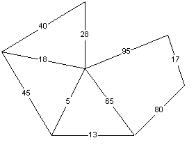
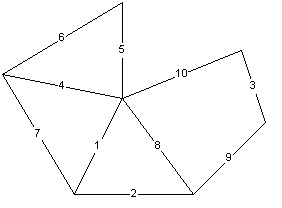
So if you have the graph:

Then the order of edges will be:

And the resulting minimal spanning tree:

This algorithm works for undirected weighted graphs.
(The prove why the algorithm works is omitted here and may be found
in any appropriated book.)
The running time of Kruskal's algorithm is O(M*logN), where M is
number of edges and N is number of nodes in graph.
"Greedy" algorithm paradigm.
Kruskal's algorithm is a good example of a greedy algorithm, in
which we make a series of decisions, each doing what seems best at
the time. The "local" decisions are which edge to add to the spanning
tree being formed. In each case we pick the edge with the smallest
weight that doesn't violate the definition of "spanning tree" by
completing a cycle.
Often the overall effect of the "locally" optimized decisions is
not "globally" optimum. However, the Kruskal's algorithm is one
of algorithms, for which it can be shown that the result is globally
optimal.
6.4.3.5 Shortest path find (Dijkstra's algorithm)
One of the "classic" tasks on graphs is: we have a graph (either
directed or undirected) with labels on its arcs (edges) representing
the "length" of each arc (edge). (Just recall the 1st example of
graph - map of roads.) The task is to find the "shortest" path
(or minimal "distance") between 2 nodes. The "distance" may have
various meaning for each particular task, even for the original
task on road map graph, such a "distance" may be: geographical
distance, time to go, cost of the way, etc.
Anyway the distance is the sum of the labels on arcs (edges)
along the path. The minimal distance from node u to node v is
the minimum of the distance of any path from u to v.
One of the algorithms solving this problem is Dijkstra's algorithm.
It finds the minimal distance from one given node (source
node) to all other nodes of the graph. So, if the desired result
is the distance from one node u to another node v, then the solution
is to apply Dijkstra's algorithm with u as the source node and stop
when it deduces the distance to v.
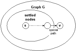
During its work the algorithm will find the minimal distance from
the source nodes to other nodes. So at any moment we will have some
nodes with already known minimal distances - such nodes are called
settled nodes (even in the very beginning there is one node -
our source).
Also at any moment we will have nodes, for which the minimal
distance is unknown yet (well, when the algorithm finishes
this set is empty). For these "unsettled" nodes we know so called
special path, which starts at the source node, goes through
settled nodes only and at the last step jumps out of the settled
"region" to the node.

The algorithm is:
- We maintain a value dist(u) for every node u. Also
we define a constant INFINITY, which is greater than the length of
any possible path in the graph G.
- If u is a settled node, then dist(u) is the length
of the shortest path from the source node s to u.
- If u is not settled, then dist(u) is the length
of the shortest special path from the source node s to u.
- Initially, only the source node s is settled, and
dist(s) = 0 (the path from s to itself). All arcs
going out from s are now special paths, so if there is an
arc from s to u, then dist(u) is the label
on the arc (its length). For all other nodes (not having arc from
s to them) we set dist(u) = INFINITY.
- Now we perform the algorithm itself. Suppose we have some settled
and some unsettled nodes. We find the node v, which is
unsettled but has the smallest dist value of any unsettled
nodes. Then we "settle" the node v by:
- Accepting dist(v) as the minimal distance from s
to v.
- Adjusting the value of dist(u) for all nodes u
that remain unsettled:
- if there is no arc v -> u - nothing to do;
- if there is such an arc, then if the sum of dist(v) and
label of the arc is less than dist(u) then we replace
dist(u) by that sum.
This step is repeated until there is no unsettled node anymore.
So if we take our example of Israel cities and distances along the
roads between them:

Then the steps of Dijkstra's algorithm for the source node Herzelia
will be as in the table below. This table represents values of
dist(u) on each step (values changed on a step are shown in
bold):
|
|
Step 1
|
Step 2
|
Step 3
|
Step 4
|
Step 5
|
Step 6
|
Step 7
|
Step 8
|
Step 9
|
Step 10
|
|
Ashdod
|
INFINITY
|
INFINITY
|
40
|
40
|
40
|
40
|
40*
|
40*
|
40*
|
40*
|
|
Beer-Sheva
|
INFINITY
|
INFINITY
|
108
|
108
|
108
|
108
|
108
|
108
|
108
|
108*
|
|
Hadera
|
INFINITY
|
28.5
|
28.5
|
28.5
|
28.5
|
28.5*
|
28.5*
|
28.5*
|
28.5*
|
28.5*
|
|
Haifa
|
INFINITY
|
INFINITY
|
INFINITY
|
INFINITY
|
INFINITY
|
79.5
|
79.5
|
79.5
|
79.5*
|
79.5*
|
|
Herzelia
|
0*
|
0*
|
0*
|
0*
|
0*
|
0*
|
0*
|
0*
|
0*
|
0*
|
|
Jerusalem
|
INFINITY
|
INFINITY
|
61
|
57
|
57
|
57
|
57
|
57*
|
57*
|
57*
|
|
Netania
|
22
|
22
|
22
|
22
|
22*
|
22*
|
22*
|
22*
|
22*
|
22*
|
|
Petakh-Tikva
|
INFINITY
|
8.5
|
8
|
8*
|
8*
|
8*
|
8*
|
8*
|
8*
|
8*
|
|
Raanana
|
0.5
|
0.5*
|
0.5*
|
0.5*
|
0.5*
|
0.5*
|
0.5*
|
0.5*
|
0.5*
|
0.5*
|
|
Tel-Aviv
|
3
|
3
|
3*
|
3*
|
3*
|
3*
|
3*
|
3*
|
3*
|
3*
|
6.4.3.6 Clique find. NP-complete tasks.
First of all, a couple of definitions more:
- A graph is called complete if all its nodes are connected to all other nodes in the graph.
- A maximal complete subgraph of a graph is a clique. The
size of the clique is the number of nodes in it.
There is an important task, which can be formulated so:
- What is the size of a largest clique in the graph?
This task is called maximum clique problem.
A corresponding decision problem is to determine whether graph G has
a clique of size k (for some given k). ("Corresponding" means that
if we can solve one of the tasks then we can solve another task as
well.)
Let's look at an example when this problem must be solved. Let's
take another aspect of planning problem: we have a set of tasks
(nodes) and dependencies between them (edges). The existence of
a dependence between 2 tasks means that these 2 tasks can not be
performed simultaneously. Also suppose that all tasks have the
same duration and there is no limitation on number of simultaneously
performed independent tasks. Now we can solve the problem by building
another graph: we create an edge between nodes, where was no edge
(dependence), and we remove edge between previously connected nodes.
So we get graph of task "independence". Now we can find the maximum
clique in this graph - the nodes in this clique will be the tasks,
which we will perform first. Then we delete the found clique from
our graph and repeat the maximum clique find for the rest of graph,
an so on.
Here is the end of good news. Bad news are that there is no known
polynomial time deterministic algorithm for this problem. Some
important notes:
- "Deterministic" - is the type of all algorithms we had in this
course. For the more scientific researches the theory of algorithms
(also called "complexity theory") has "nondeterministic" algorithms
as well, but they are out of scope of this course.
- "Polynomial time" - means O(p(N)), where p(N) is any polynom
of N, i.e. a0N + a2N2 + ... +
akNk. What does it mean that there is no such
an algorithm? It means that the only known way to solve the problem
is to try all the possibilities, i.e. all possible subgraphs, i.e.
the time will be O(2N) - it is clear that this function
grows much faster than any polynom.
- "There is no known" - means that it is not proven that there is
no such an algorithm, but it is not found yet, moreover its existence
seems unlikely, at least because of the huge effort that has already
been expended by very many people on this and similar problems.
Another such problem is so called Travelling Salesman Problem:
you have a graph of cities and roads between them, you have a salesman,
who have to visit some of the cities, each city once only. You must
find the best (e.g. shortest) way for the salesman. This "simple" task
is also not solvable in polynomial time.
Such problems are called NP-complete. There are 14 known
NP-complete problems; list of them may be found in any appropriate
book. The number 14 means that there are 14 REALLY different problems,
but there is a lot of problems, which may be transformed to one of
these 14 (like our 2 variants of clique task). Once again: it is
not proven that they are not solvable in polynomial time, but there
is no such a solution known.
It is very important, when you try to solve some particular problem,
to check: perhaps the problem is NP-complete? If it is then it may
be solved for very small size only, and you have to find another
approach for solution (may be not exact but some approximate
solution?).
6.5 Important graph applications
Among other examples of graph application there is a lot tasks more,
where graphs are the best (and often the only) way to solve them. In
fact any task, where you have some instances and binary relationship
between them, seems to be represented by graphs in the most handy
and clear way. There is indefinite amount of such examples:
- Internet sites and references between them - an analysis used
by some Internet search engines.
- People with any relationship between them (say, friendship) - an
analysis used in psychology.
- Atoms and bonds between them - an analysis used in chemistry.
- etc. etc. etc.
Some of such representations are so important that they have
wide field of application and even their own names.
For example, if you have some system (system may be a physical
system, or program, or whatever else), which at any moment can
be in one of some definite states, and you know all possible
transformations of the system from a state to another state, then
the best representation of such a system is so called Finite
State Machine: a graph with nodes - possible states, and arcs -
possible transformations between states.
As a conclusion: a graph theory is a vast science, and this course
touched the very basic issues only. Anyway having the understanding
of the main approaches and possible problems here should help to
find solutions for the real specific tasks (for example, in books).
