1. Purely Competitive Firms - accepts the market price in order to sell their products.  They are also called price takers.
   • Characteristics:
     • All firms produce an identical product
       • Consumers do not care where they buy the product
     • A large number of firms are in the market
     • Each firm supplies only a small portion of the total supplied to the market
       • One firm cannot influence the price of the market
     • No barriers to entry or exit exist
       • Example:  If one firm earns economic profit, then rival firms can easily enter the market and try to earn profits
     • The firms maximize profit by adjusting production level, but cannot influence market price.
2. Why study price takers?
   • Understand why competition is important
   • Clarifies differences between price-takers and other firm types
   • Agricultural markets tend to be price takers

1. Marginal Revenue (MR) - is the change in total revenue when output increases by one unit.

• Refer to graph.
• The farmer only sees the market price.
  • If the farmer sells 1 bushel, he receives $2 (MR).  The farmer sells another bushel, he receives another $2 (MR).
  • If the farmer raises his price of corn above the market price, then nobody buys it.
    • Consumers buy the bushel from competitors for $2
  • If the farmer sells his corn below the market price, then he lowers his revenue (loses money)
  • Thus, he can sell all his corn at the market price, so MR = P* = $2.

Price Taker's Demand Curve
A Farmer	The Market
Price	Price
Quantity	Quantity

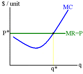
2. Profit maximization - the price taker will expand output in the short run until:

P* = MR = MC

Note: The market price is P* and marginal cost is MC. Further, the MR = MC maximizes profits for monopolies, oligopolies, and monopolistically competitive firms, while MR = P* is only valid for price takers.
 

	This rule maximize the firm's profits (or minimize its losses)
	Example: If MR = $3 and MC = $2. MR > MC, the firm will collect $3 for selling that last "additional" unit that only costs $2 to produce. Profit increases by $1. If MR = $3 and MC = $5. MR < MC, the firm will collect $3 for selling that last unit that costs $5 to produce. The firm should reduce production by 1 unit to increase profits.

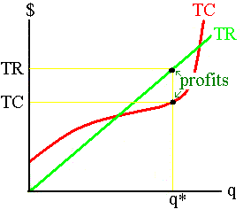
• Price takers earn profits by maximizing total revenue (TR) and minimizing total costs(TC)
  • Total Revenue (TR) = P * q
  • Profits = TR - TC
  • Taking vertical slices (adjusting output q) until TR -TC is maximized, which is shown below:

Firm
Price / Per-unit costs
The point where profit is maximized is at the production level q when MC = MR = P*
Quantity

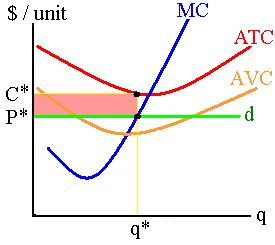
• Using the marginal cost, market price, and average total cost, we can show a competitive firm earning a profit.
  • Firm earns a profit when Market Price > ATC
  • The "green" rectangle is firm's profit
• The derivation is:

Profit = Total Revenue - Total Cost

Profit = P q - ATC q = (P - ATC) q

Firm
Price / Per-unit costs
Quantity

3. Losses and going out of business.

• Short-run.
  • A firm experiencing losses, but covering its average variable costs, will operate in the short run.
  • Example: AVC = $10 per product, AFC = $10, and the firm produces where MR = MC.
    • Competitive market: P* = MR 
      •  If P* = $5; firm cannot cover its variable costs, so it shuts down; it still pays its fixed costs
      • If P* = $10; firm covers its variable costs, but earns a loss
      • If P* = $15; firm still earns a loss, but also covers some of its fixed costs
      • If P* = $20; firm breaks even
      • If P* > $20; firm earns an economic profit
  • Shutdown - temporary halt in the production or operation of a business.
    • A firm shuts down when P* < AVC
    • The firm still pays fixed costs during the shutdown.
    • Motels, restaurants, and theme parks shutdown during off seasons 
• Long-run.
  • A firm will "go out of business" in the long run whenever P < ATC.
  • Going out of business - firm permanently exits the market and avoids paying fixed costs.
    • If P = $0.25 for a generic soda and the ATC = $0.50.
    • This firm cannot continue to operate for a long time with losses.

	A Firm
	Price / Per-unit costs
Firm produces quantity q where MC = MR = P ATC > Market Price, the firm is earning a loss or profit is negative. Profit = Total Revenue - Total Cost Profit = P q - ATC q The loss = "The red area"
	Quantity

4. A firm maximizes profits when it produces at P* = MC. A firm's short-run supply curve is its marginal cost curve above average variable cost.  Firm produces if the market price exceeds its average variable costs.

Law of Supply - as the price of a product increases, firms will increase quantity supplied.

A Firm's Cost Curves	A Firm's Supply Curves
Price / Per-unit costs	Price / Per-unit costs
Quantity	Quantity

• In the long-run, firms earn zero economic profit
  • A normal rate of return, i.e. accounting profit
• If P* > ATC, firms earn an economic profit
  • New firms enter the market
  • SR Supply increases while the price decreases until it equals P = ATC
  • Economic profit = 0
• If P* < ATC, firms earn a loss
  • Some firms leave the market
  • SR supply decreases, while the price increases until it equals P = ATC
  • Economic profit = 0
• Long-run equilibrium
  • The market determines the price and quantity of milk
    • P* = $2 and market quantity = 10 (thousand)
  • Each firm supplies q quantity of milk
    • Earn zero economic profit
    • P* = ATC = $2

A Milk Firm's Long-Run Cost Curve	The Milk Market
Price / Per-unit costs	Price / Per-unit costs
Quantity	Quantity (in thousands)

• Example: The U.S. Gov. says drinking milk does the body good
  • Consumers start buying more milk (tastes and preferences)
    • The demand curve shifts right.
      • New market price is P₂
      • Quantity supplied and sold is Q₂
  • Firms expand output to q₂
    • Earn economic profits (P₂ > ATC)
  • Long-run equilibrium
    • New firms enter the milk market
    • Short-run supply increases
    • Price decreases, until P₁ = ATC again
  • Result:
    • Same market price, P₁
    • More milk produced and sold, Q₃
    • More firms are in the market and all earn zero economic profit

A Milk Firm's Long Run Cost Curve	The Milk Market
Price / Per-unit costs	Price / Per-unit costs
Quantity	Quantity

• Economic losses and exit
• Example: Consumers' income increases and rice is an inferior product
  • The original demand & supply curves are D₁ & S₁
  • Demand curve shifts left.
    • New market price is P₂
    • Quantity supplied and sold is Q₂
  • Firms contract output to q₂
    • Earn economic losses (P₂ < ATC)
  • Long-run equilibrium
    • Some firms leave the rice market
    • Short-run supply decreases
    • Price increases, until P₁ = ATC again
  • Result:
    • Same market price, P₁
    • Less rice produced and sold, Q₃
    • Less firms are in the market and all earn zero economic profit

A Firm Producing Rice	The Rice Market
Price / Per-unit costs	Price / Per-unit costs
Quantity	Quantity

Long run supply - the minimum price which firms will supply various production levels when all factors of production can be adjusted. The long-run supply is the black lines in the milk and rice markets

1. Constant-cost industry - industry were resource prices remain unchanged as market output is expanded
   • Long-run market supply curve is horizontal (perfectly elastic)
   • Illustrated above in milk and rice markets
   • An expanding/contracting industry has no impact on the resource markets, because it is a small industry
2. Increasing-cost industry - industry were factor prices rise as market output is expanded
   • Long-run market supply curve is upward-sloping
   • Most common type of industry
   • Example: If automobile factory expands production, then resource prices will increase: skilled labor, steel, plastics, etc.
3. Decreasing-cost industry - industry were factor prices decline as market output is expanded
   • Long-run market supply curve is downward-sloping
   • Rare type of industry
   • Example: Electronic industry. As more and more transistors are etched onto chips, then cost of chips, computers, etc. keep decreasing

Automobile Firm - Increasing Costs	Computer Chip Firm - Decreasing Costs
Price	Price
Quantity	Quantity

P₁ and Q₁ are the original demand and supply curves for both markets. Consumer demand more cars and electronics, because of higher incomes. The new market price is P₂. Both industries earn economic profits, which cause them to expand.

As car industry expands, the resource prices increase (skilled labor, steel, etc.), causing the long-run price and quantity to be P3 and Q3. As the electronic industry expands, the resources prices decrease (computer chips), causing long-run price and quantity to be P3 and Q3.

• Profit is a reward for increasing the value of resources.
  • total revenue (consumers' valuation) > total costs (firm's costs of resources).
    • Minimize costs
    • Operate efficiently
    • Innovate
    • Weeds out inefficient firms
    • Satisfy consumers
• Losses are a penalty imposed on firms that reduce the value of resources.
  • Firm will either leave the market, restructure, or bankrupt.
• Competitive market is efficient
  • Allocative efficiency - businesses transfer resources to profitable industries that consumers want
    • P* = MC
  • Productive efficiency - businesses produce products for the lowest price
    • P* = min ATC
  • Social welfare is maximized
    • Consumer plus producer welfares are maximized
• New products
  • Microwave ovens
  • Personal computers
  • DVDs / Blue Ray

Competitive markets and profits create wealth and direct resources to produce highly-valued goods.