|
|
|||||
|
|
|
|
|
|
|
|
|
|||||
|
|
|||||
|
|
|
|
|
|
|
|
|
|||||
by Evgeny Tarabrin
Any complex dynamic system can be submitted as set of the interconnected parts. The parts of system can be diversified: static, dynamic, linear, nonlinear etc.. The algorithms implimented by these parts, are defined by a subject domain, for which the modeling is carried out. The allocation of parts as separate independent elements and definition of connections between them is the main task for preparation of investigated process for modeling. The complex systems differ that the connections between parts do not remain constant, and can change during system functioning. These connections can occur or disappear during evolution of system, giving its behaviour the rather complex and confusing character and complicating its research by known methods. Practically study of behaviour of such systems with structure, varied in time, is possible only by modeling on the computer.
In present clause it is offered design pattern, allowing to simulate behaviour of complex dynamic systems with varied connections. Main in the given approach is essential use of such concepts OOP as encapsulation, inheritance and polymorphism. As base language is used Java, though with the same success the stated approach is possible to realize with the help of other OOP languages (C ++, SmallTalk etc.).
The essence of the offered approach consists in the following. At drawing up the model of system it is necessary in an obvious manner to allocate independent parts and connections between parts. Each part and each connection are represented as objects. The object-part represents algorithm of independent functioning of an element, and the object-link contains the information on what parts are connected by the given connection and what condition of this connection (active or inactive). The allocation of connection as independent object allows simply enough to manipulate a condition of connection during system modeling. In clause the appropriate classes and general procedure of system modeling of a similar sort are given.
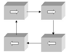
In figure 1 the generalized structure of simulated system is submitted. Here in an obvious manner the parts of system and connections between them are allocated.
|
|
|
Fig.1. |
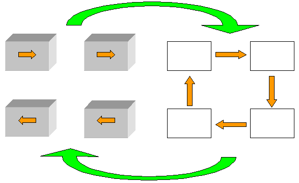
The solving of such systems is convenient to break on two stages (figure 2).
|
|
|
Fig.2. |
At the first stage of the solving it is supposed, that all connections between parts of system are broken off and there is a processing of the information inside each independent block. The essence of this processing is that the element should to calculate his output variables by using its given input variables. The order of parts processing can be any.
At the second stage of the solving there is a processing of all connections between parts of system. It means that the output value of an element is transferred to an input of other element connected by the given connection. Thus the behaviour of elements is not accepted in account on this stage. They are as though frozen.
Then the transition to the first stage of the solving is carried out and the process repeats again.
The error of such decision can be made sufficently small at enough small value of modeling step.
The functional model of a class Block is submitted in figure 3.
|
|
|
Fig.3. |
A basic element of a class is the procedure solve(), which provides processing input variables according to algorithm of work of an independent element. It is natural that this method is abstract and should be overridden in the inherited class. The separate part can have some inputs and outputs and to distinguish them for each of them own number named as inputIndex or outputIndex is nominated. The numbering of inputs and outputs begins with 0. The class has also two public methods for an establishment of values of input variables (setInput ()) and reception of values of output variables (getOutput()). It is supposed, that all input and output variables have a type float and are stored in an appropriate arrays. Listing of a class Block is given below :
abstract class Block{
    protected float[] input;
    protected float[] output;
    public void setInput(int inputIndex, float value){
        this.input[inputIndex]=value;
    }
    public float getOutput(int outputIndex){
        return this.output[outputIndex];
    }
    abstract public void solve();
}//end class Block
In figure 4 the structure of an abstract class Block together with the several inherited classes for concrete elements of a system is submitted.
|
|
|
Fig.4. |
From here it is clear, what there should be a structure of a class expanding an abstract class Block. Each of the inherited classes includes a set of the constructors for creation of object with those or other properties and overriden method solve() determining algorithm of functioning of an element.
In this section the mathematical models of some typical elements and classes appropriate to them and expanding a base abstract class Block are submitted. The purpose of these examples - to show a technique of drawing up of classes for modeling concrete elements of system. The presence of the several constructors is rather useful as allows to reflect various aspects of created objects.
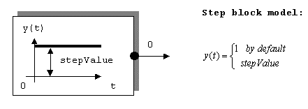
In figure 5 a model for a step signal is submitted.
|
|
|
Fig.5. |
class StepBlock extends Block{
    private float stepValue=1.0f;
    public StepBlock(float stepValue){
        this.stepValue=stepValue;
        output=new float[1];
        output[0]=stepValue;
    }
    public StepBlock(){
        output=new float[1];
        output[0]=stepValue;
    }
    public void solve(){};
}//end class StepBlock
In figure 6 a model for aperiodic element is submitted.
|
|
|
Fig.6. |
class AperiodicBlock extends Block{
    private double T=1.0;
    public AperiodicBlock(double T){
        this.T=T;
        input=new float[1];
        input[0]=0.0f;
        output=new float[1];
        output[0]=0.0f;
    }
    public AperiodicBlock(){
        input=new float[1];
        input[0]=0.0f;
        output=new float[1];
        output[0]=0.0f;
    }
    public void solve(){
        output[0]=output[0]+(float)((Environment.dt/T)*
        (input[0]-output[0]));
    }
}//end class AperiodicBlock
In figure 7 a model for summing element is submitted.
|
|
|
Fig.7. |
class SumBlock extends Block{
    private int g0=1;
    private int g1=1;
    public SumBlock(int g0,int g1){
        if(g0>=0) this.g0=1;
        else this.g0=-1;
        if(g1>=0) this.g1=1;
        else this.g1=-1;
        input=new float[2];
        input[0]=0.0f;
        input[1]=0.0f;
        output=new float[1];
        output[0]=0.0f;
    }
    public SumBlock(){
        input=new float[2];
        input[0]=0.0f;
        input[1]=0.0f;
        output=new float[1];
        output[0]=0.0f;
    }
    public void solve(){
        output[0]=(float)(g0*input[0]+g1*input[1]);
    }
}//end class SumBlock
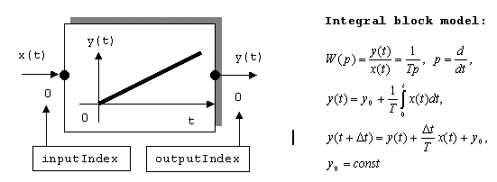
In figure 8 a model for integrator element is submitted.
|
|
|
Fig.8. |
class IntegralBlock extends Block{
    private double T=1.0;
    private double Y0=0.0;
    public IntegralBlock(double T){
        this.T=T;
        input=new float[1];
        input[0]=0.0f;
        output=new float[1];
        output[0]=0.0f;
    }
    public IntegralBlock(){
        input=new float[1];
        input[0]=0.0f;
        output=new float[1];
        output[0]=0.0f;
    }
    public IntegralBlock(double T,double Y0){
        this.T=T;
        this.Y0=Y0;
        input=new float[1];
        input[0]=0.0f;
        output=new float[1];
        output[0]=0.0f;
    }
    public void solve(){
        output[0]=(float)(Y0+output[0]+(Environment.dt/T)*input[0]);
    }
}//end class IntegralBlock
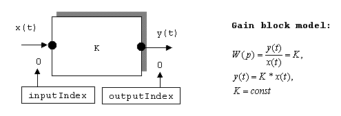
In figure 9 a model for an element with constant gain of amplification is submitted.
|
|
|
Fig.9. |
class GainBlock extends Block{
    private float k=1.0f;
    public GainBlock(float k){
        this.k=k;
        input=new float[1];
        input[0]=0.0f;
        output=new float[1];
        output[0]=0.0f;
    }
    public GainBlock(){
        input=new float[1];
        input[0]=0.0f;
        output=new float[1];
        output[0]=0.0f;
    }
    public void solve(){
        output[0]=(float)(k*input[0]);
    }
}//end class GainBlock
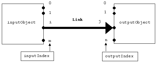
The functional model of a class Link is submitted in figure 10.
|
|
|
Fig.10. |
Each separate object of a class Link connects one of outputs of the inputObject and one of inputs of the outputObject. As already was spoken earlier, variable inputIndex defines number of an output of the inputObject, and variable outputIndex defines number of an input of the outputObject.
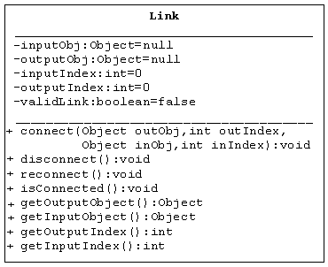
In figure 11 the structure of a class Link is submitted.
|
|
|
Fig.11. |
Attributes of this class contain private references to the connected objects and also number of inputs and outputs of these objects. The default constructor creates object-link with the empty references. The concrete values to the references will be assined with the help of a method connect(). The class Link has a set of methods for manipulation with object-link. With the help of a method disconnect() it is possible to break off connection (thus object-link is kept in memory !). To restore connection it is possible with the help of a method reconnect(). The method isConnected() serves to check a condition of the onnection. The set of methods getXXX() allows to receive the information on the connected objects.
The complete description of a class Link is given below:
class Link{
    private Object inputObj=null;
    private Object outputObj=null;
    private int inputIndex=0;
    private int outputIndex=0;
    private boolean validLink=false;
    public void connect(
      Object outObj,int outIndex,Object inObj,int inIndex){
        this.inputObj=inObj;
        this.inputIndex=inIndex;
        this.outputObj=outObj;
        this.outputIndex=outIndex;
        this.validLink=true;
      }
    public void disconnect(){this.validLink=false;}
    public void reconnect(){this.validLink=true;}
    public boolean isConnected(){return validLink;}
    public Object getOutputObject(){return outputObj;}
    public Object getInputObject(){return inputObj;}
    public int getOutputIndex(){return outputIndex;}
    public int getInputIndex(){return inputIndex;}
}//end class Link
This class is convenient for a storage of the various information about process of modeling. In the given example in this class is determined static variable dt, representing a time interval for one step of modeling. The description of a class Environment is given below:
class Environment{
    public static double dt;
}//end class Environment
1. Modeling aperiodic element reaction on step signal.
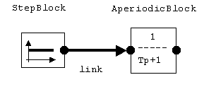
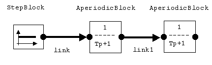
In figure 12 the system consisting from two elements is submitted:
-element forming a step signal,
-element simulating aperiodic block.
|
|
|
Fig.12. |
The program of the solving of this task is submitted by a class Solver in a file Solver.java. The constructor of the class Solver() contains the information on a concrete task and for each example will be various.
public class Solver{
    public Solver(){
        Environment.dt=1.0;//time-step of modeling
        StepBlock step=new StepBlock();
        AperiodicBlock aper=new AperiodicBlock(7.0);
        Link link=new Link();
        link.connect(step,0,aper,0);
        Vector dynBlocks=new Vector();
        Vector links=new Vector();
        dynBlocks.addElement(step);
        dynBlocks.addElement(aper);
        links.addElement(link);
        for(int i=0;i<21;i++)
        {
            stageOne(dynBlocks);
            stageTwo(links);
            System.out.println(i+"  "+aper.getOutput(0));
        }//end for loop
        try//to delay on the screen
        {
            System.in.read();
        }
        catch(IOException e){}
    }//end Solver()
    public static void main(String[] args){
    Solver solver=new Solver();
    }//end main()
    private void stageOne(Vector dynBlocks){
        Enumeration dynBlEn=dynBlocks.elements();
        while(dynBlEn.hasMoreElements()){
            Object aDynBlock=dynBlEn.nextElement();
            ((Block)aDynBlock).solve();
        }//end while loop
    }//end stageOne()
    private void stageTwo(Vector links){
        Enumeration linksEn=links.elements();
        while(linksEn.hasMoreElements()){
            Object aLink=linksEn.nextElement();
            Block outBlock=(Block)(((Link)aLink).getOutputObject());
            int outInd=((Link)aLink).getOutputIndex();
            Block inBlock=(Block)(((Link)aLink).getInputObject());
            int inInd=((Link)aLink).getInputIndex();
            inBlock.setInput(inInd,outBlock.getOutput(outInd));
        }//end while loop
    }//end stageTwo()
}//end class Solver
The class Solver contains two private methods - stageOne() and stageTwo() which realize two-stage logic of modeling described above. In these methods is significally used polymorphism via methods calls.
The object dynBlocks type of Vector contains the information on all elements participating in process.
The object links type of Vector contains the information on all connections between elements of system. Used polymorphism extremely simplifies realization of process modeling. In a method stageOne() all elements are simply taken on turn and for each of them the appropriate realization of a method solve() is used. In a method stageTwo() all objects-links are serially taken and the transfer of value from an output of the inputObject on an input of the outputObject is made for each of them.
The method main () serves for creation of object of a class Solver.
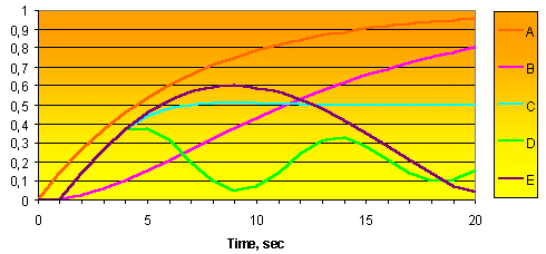
The result of modeling of the given example is submitted as a curve A in figure 13 (Taper=7.0 sec).
|
|
|
Fig.13. |
2. Modeling two consiquently connected aperiodic elements reaction on step signal.
In figure 14 the modeling circuit for the given example is submitted.
|
|
|
Fig.14. |
The description of the constructor of a class Solver for the solving of this task is given below. All other classes remain without change.
The result of modeling is submitted as a curve B in figure 13 (Taper1=Taper2=7.0 sec).
public Solver(){
        Environment.dt=1.0;
        StepBlock step=new StepBlock();
        AperiodicBlock aper=new AperiodicBlock(7.0);
        AperiodicBlock aper1=new AperiodicBlock(7.0);
        Link link=new Link();
        Link link1=new Link();
        link.connect(step,0,aper,0);
        link1.connect(aper,0,aper1,0);
        Vector dynBlocks=new Vector();
        Vector links=new Vector();
        dynBlocks.addElement(step);
        dynBlocks.addElement(aper);
        dynBlocks.addElement(aper1);
        links.addElement(link);
        links.addElement(link1);
        for(int i=0;i<21;i++)
        {
            stageOne(dynBlocks);
            stageTwo(links);
            System.out.println(i+"  "+aper.getOutput(0)+"  "+aper1.getOutput(0));
        }//end for loop
        try
        {
            System.in.read();
        }
        catch(IOException e){}
    }//end Solver()
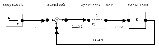
3. Modeling proportional regulation of the aperiodic object.
In figure 15 the modeling circuit for the given example is submitted.
|
|
|
Fig.15. |
The description of the constructor of a class Solver for the solving of this task is given below. All other classes remain without change.
The results of modeling are submitted in figure 13 as a curve C (Taper=7.0 sec, K=1.0) and D (Taper=7.0 sec, K=4.0). The shift of the diagrams in the beginning of process on value of dt=1.0 sec demonstrates influence of a time interval for one step of modeling on accuracy of the modeling.
To increase the accuracy of modeling the value of the dt should be reduced.
public Solver(){
        Environment.dt=1.0;
        StepBlock step=new StepBlock();
        SumBlock sum=new SumBlock(1,-1);
        AperiodicBlock aper=new AperiodicBlock(7.0);
        AperiodicBlock aper1=new AperiodicBlock(7.0);
        GainBlock gain=new GainBlock(4.0f);
        Link link=new Link();
        Link link1=new Link();
        Link link2=new Link();
        Link link3=new Link();
        link.connect(step,0,sum,0);
        link1.connect(sum,0,aper,0);
        link2.connect(aper,0,gain,0);
        link3.connect(gain,0,sum,1);
        Vector dynBlocks=new Vector();
        Vector links=new Vector();
        dynBlocks.addElement(step);
        dynBlocks.addElement(sum);
        dynBlocks.addElement(aper);
        dynBlocks.addElement(gain);
        links.addElement(link);
        links.addElement(link1);
        links.addElement(link2);
        links.addElement(link3);
        for(int i=0;i<21;i++)
        {
            stageOne(dynBlocks);
            stageTwo(links);
            System.out.println(i+"  "+aper.getOutput(0));
        }//end for loop
        try
        {
            System.in.read();
        }
        catch(IOException e){}
    }//end Solver()
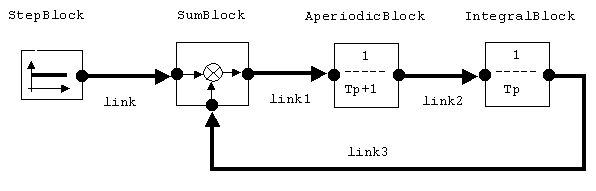
4. Modeling integral regulation of the aperiodic object.
In figure 16 the modeling circuit for the given example is submitted.
|
|
|
Fig.16. |
The description of the constructor of a class Solver for the solving of this task is given below. All other classes remain without change.
The result of modeling is submitted as a curve E in figure 13 (Taper=7.0 sec, Tint=5.0 sec).
public Solver(){
        Environment.dt=1.0;
        StepBlock step=new StepBlock();
        SumBlock sum=new SumBlock(1,-1);
        AperiodicBlock aper=new AperiodicBlock(7.0);
        IntegralBlock integral=new IntegralBlock(5.0);
        Link link=new Link();
        Link link1=new Link();
        Link link2=new Link();
        Link link3=new Link();
        link.connect(step,0,sum,0);
        link1.connect(sum,0,aper,0);
        link2.connect(aper,0,integral,0);
        link3.connect(integral,0,sum,1);
        Vector dynBlocks=new Vector();
        Vector links=new Vector();
        dynBlocks.addElement(step);
        dynBlocks.addElement(sum);
        dynBlocks.addElement(aper);
        dynBlocks.addElement(integral);
        links.addElement(link);
        links.addElement(link1);
        links.addElement(link2);
        links.addElement(link3);
        for(int i=0;i<21;i++)
        {
            stageOne(dynBlocks);
            stageTwo(links);
            System.out.println(i+"  "+aper.getOutput(0));
        }//end for loop
        try
        {
            System.in.read();
        }
        catch(IOException e){}
    }//end Solver()
|
|
|
|
|
|
|
Copyright © 2000 Evgeny Tarabrin