The effects of consumer preference heterogeneity and market entry fixed costs on the stability of a duopol market

- The network externalities approach

a Monte-Carlo simulation case study

by
Csaba Horváth
June, 1999

Contact:
m42@iname.com
http://www.oocities.org/wallstreet/9403

A concept of network externalities

According to the basic network externality model, the utility that a subscriber derives from a product increases as more and more other users starting to use the same product. Namely, the consumers’ valuation of a brand increases with the number of other consumers using the same brand. Typical examples are telecommunication and operating systems.

The structure of the Monte-Carlo simulation

The market structure

We assume a duopol market that is symmetric at the beginning. The number of consumers starts from a certain number (denoted as „!oldusers” in the program) on each side, other number of „!nuser” users buy one of the two brands consequitively. Consumers decide upon buying one of the brands. The two brands are ‘WIN’ and ‘MAC’ (only for the sake of simplicity :-)). Three factors are taken into account by the consumers when deciding which brand to choose:

The winner is the firm which gains a given (!rulezlimit) market ration before the market gets saturated.

The market grows from !oldusers to !oldusers*2+!nusers.

The variables are calculated at each step as follows:

The decision algorithm of the consumers

Consumers compare the utility of the two brands. The preference of the consumers is defined by the variable „!actualuserpref” during the simulation. Preferences vary from 0 to „!hetero” with a uniform distribution, where „!hetero” stands for the heterogeneity of the consumers (a higher value denotes a higher degree of variability in preferences). The consumers decide one after another, they buy the brand with the higher utility for them. Formally:

!winutil=(!ratio)*(!hetero-!actualuserpref)-@sqrt((!pwin/!pmac))
!macutil=(1-!ratio)*(!actualuserpref)-@sqrt((!pmac/!pwin))
if !winutil>!macutil then !nwinuser=!nwinuser+1
else
!nmacuser=!nmacuser+1
endif

After each entrant, the market share, prices and costs are recalculated, after which the next consumer enters to the market. The process (that is one simulation) comes to end when one of the firm reaches a market share of 85% OR there are 300 consumers on the market.

See appendix or http://www.oocities.org/wallstreet/9403/mktshare.htm for the source code.

Scenarios

We examine nine scenarios in two dimensions. The two dimensions are:

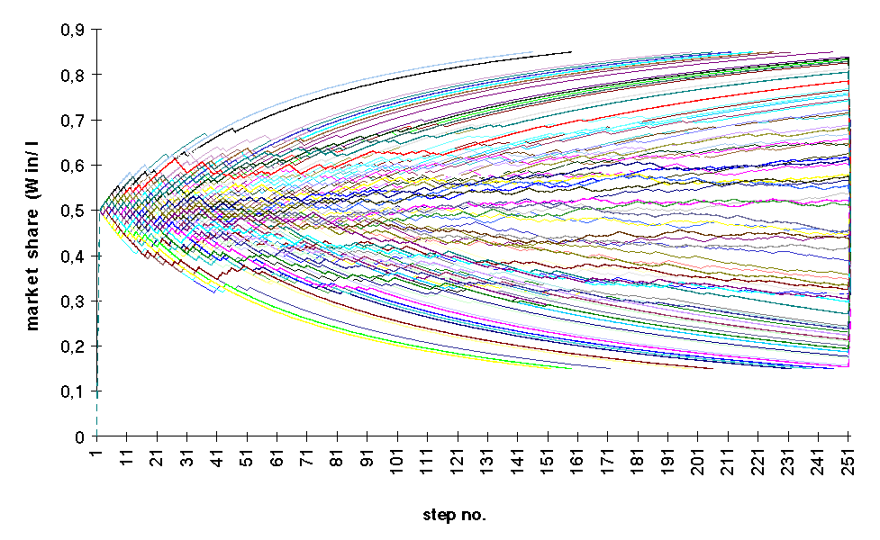
Three cases in two dimensions means 9 cases. Each time 100 simulations were conducted.

Results of the simulations

A simulation can be observed and analysed from a number of different points of view. Our program allows you to do different types of what-if analyses, but now – for the sake of shortness – we are confined to the evolution of the market share.

Firstly, we take the case of a middle course: heterogeneity of value 2 and fixed cost of value 250. The picture below show the results of the simulations.

Figure A: Evolution of market shares during the simulations
(consumer heterogeneity: intermediate, fixed costs: intermediate (hetero=2, fc=250))

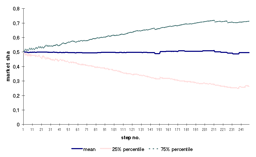
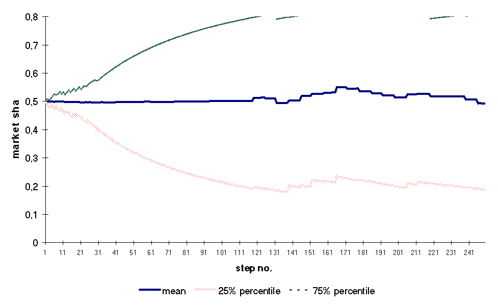
The picture above gets messy if we increase the number of simulations. For that reason we concentrate only on the main tendecies, and we do that by keeping an eye on the evolution of say 25^th and 75^th percentiles.

Figure B: 25^th and 75^th percentiles of market shares during a simulation
(consumer heterogeneity: intermediate, fixed costs: intermediate (hetero=2, fc=250))

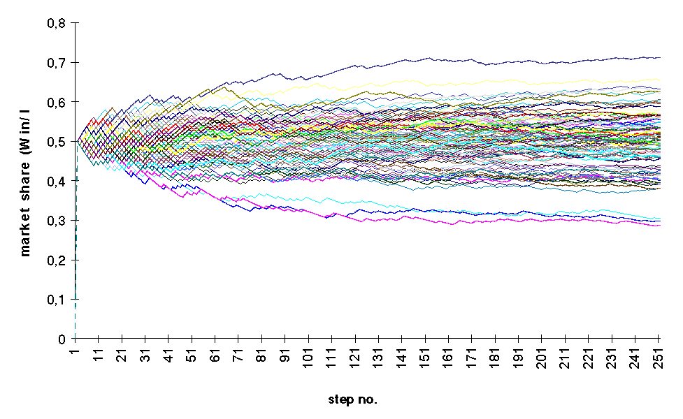
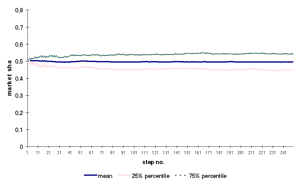
As assumed, the 50^th percentile fluctuates around 0.5. The 25^th and 75^th percentiles surround 50% of cases.

Secondly, let us consider a more extreme case: fixed cost are low (FC=100), but customer preferences are more heterogenous (HETERO=10). In this case after simulating 100 cases, the figures look like this.

Figure C: Evolution of market shares during the simulations
(consumer heterogeneity: high, fixed costs: low (hetero=10, fc=100))

Figure D: 25^th and 75^th percentiles of market shares during a simulation
(consumer heterogeneity: high, fixed costs: low (hetero=10, fc=100))

Both figure depict a more stable market structure. The reason for this is that having these paramters the difference in unit costs is less significant than before. In addition, consumers choose more „randomly”.

Thirdly we examine a case of high fixed cost and low variance in preferences.

Figure E: Evolution of market shares during the simulations
(consumer heterogeneity: low, fixed costs: high (hetero=1, fc=500))

Figure F: 25^th and 75^th percentiles of market shares during a simulation
(consumer heterogeneity: low, fixed costs: high (hetero=1, fc=500))

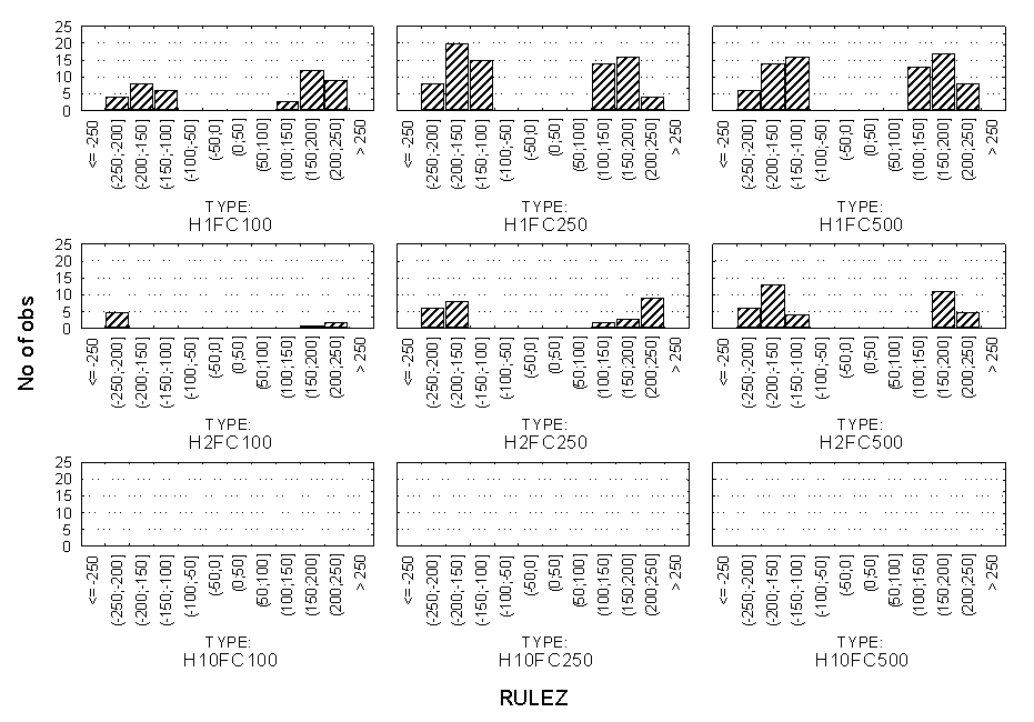
This case is the other extreme: the initial advantage often turns out to be irreversible and one of the firms obtains a ruling market share. This is because an initial advantage in market share is reflected in the costs to a great extent (because of high fixed costs) and is only slightly offset by the variability of consumer preferences.

Now we examine that in how many cases and when occurs the take-over of a market (one firm rules the market). The examples above can help us to form our judgements: higher fixed cost and lower variability in preferences contribute to the development of monopoly. This is depicted by the following figure.

Figure G: Categorised histogram: the distribution of take-over points during the simulations in 9 different market structure setups (negative values mean WIN monopoly, posivie values stand for MAC monopoly)

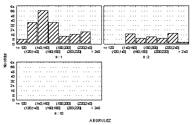
Concentrating on the take-over points, we examine the relationship between consumer preference heterogeneity and the probability of development of a monopoly. For that purpose we plot against the measure of variability in preferences (H= 1, 2, 10) and the histogram of take-over points.

Figure H: The relationship between consumer preference heterogeneity and the probability of development of a monopoly.

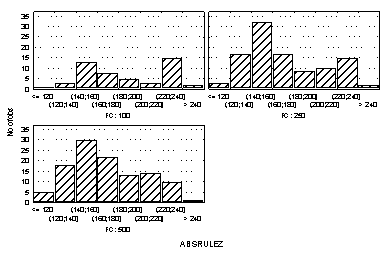
An evidence was found that a lower degree of variability in preferences contributes to a higher chance of development of a monopoly (both during a game and in an earlier case). On the above picture horizontal axis indicates the phase of monopolisation perion (variable „ABSRULEZ”).

We still concentrating on the take-over points. At this point we examine the relationship between fixed costs and and the probability of development of a monopoly. Let us plot against the measure of fixed costs (FC= 100, 250, 500) and the histogram of take-over points.

Figure I: The relationship between initial fixed costs and the probability of development of a monopoly.

One can easily determine that high fixed cost make the polarized market structure unstable. On the opposite, low fixed costs support a duopoly.

Conclusion

The aim of this short paper was to build a general simulation framework where the relationship between different market properties (economies of scale, market size, consumer loyalty, variance in preferences, level of fixed costs) and the stability of a duopol market structure can be simulated simultaneously.

We examined the effect of fixed costs and of the variability in consumer preferences.

We found that a lower variability in consumer preferences and higher fixed cost encourage the monopolisation of the market: one of the firms takes over the market with a higher probability and in an earlier step.

The simulation framework can be modified and extended easily for any Monte-Carlo simulation and calibration purposes.

Appendix: Source Code in EViews programming language

The program code (MKTSHARE.PRG) and initial Eviews workfile (MKTSHARE.WF1) are available in a single zipped file (MKTSHARE.ZIP).

Instructions: download the MKTSHARE.ZIP file to your computer, and open it with your favourite ZIP shell.

Literature