|
Once more, the purely geometric analysis of the phenomenon is essential for understanding the wave behavior. Let us pinpoint the deformations the wavefront undergoes as a structure of the Schild space-time when it moves in a resonance orbit, and observe in quantum-dimensional terms what happens along the orbit of length: l = 2pr. The linear quantum L constitutes, as we have seen, the modulus composing any distance, and the resonance orbit must be therefore formed by an integer of linear quanta L. Following step by step the propagation of the surface quantum L2 , which is in the orbit in a resonance condition, seeing that it is an elementary component of wavefront, we can ascertain that after covering a certain distance nL, (with n as an integer) the surface quantum L2 produces a new perturbation surface multiplying itself according to the modalities of the Schild space-time.
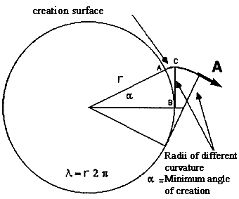
Where the radii of curvature of the different produced surface portions are identified with the vector A that develops on the plane described in the plane involute formula 66) that we call: AE.The reason for the production of a new perturbation surface is justified by the change in horizon which the wavefront moving in resonance conditions is subjected to. When a wavefront in the resonance orbit describes an arc having an angle a, the projection of the previously started perturbation has described a straight line path. We can verify it from the geometric construction and from the necessary conditions for the creation of the involute curve. Let us suppose that the resonant wavefront is perpendicular to the orbital curve. Then, simplifying the mathematical handling, let us consider the arc subtended to the angle a as a rectilinear segment; finally, given the exiguity of its length compared to the resonance orbit, let us consider the straight triangle ABC, in Fig. 20.Let us use the phytagorean theorem in order to find the value AE . 71) A2E = (r + L)2 - r2 from which it follows that A2E = 2rL + L2 Let us leave out L2 seeing that is a negligible distance compared to r. 72)
73)
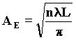
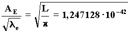
74) l = l e is: AE = 1,942607 10-48 m This is the length of the vector that is approximately identified with the arc described by the resonant wavefront in order to create a new surface quantum L2 during its propagation along the electron's resonance orbit. The ratio between the length AE of the arc necessary for the creation of a new surface on the resonance orbit and the root of the primary wavelength is: 76)
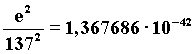
Such a ratio is a constant fundamental characteristic of the spherical involute model so that a particle can be defined elementary only if its creation ratio of perturbation remains unchanged with time, and it is “perhaps” in connection with the electric charge. 77)
On each wavefront created by the involute, which go away from the resonance orbit, there will be some surface adjacent portions endowed with different radii of curvature. The passage from a curvature to the immediately upper one occurs by jumps because, as we have seen above, the radius of curvature increases only by discrete quantities. Along the whole almost spherical wavefront of the involute, from the origin on the orbit till the infinity, there will be some increasing lenght sectors of wavefront with different curvature. The equatorial curve of the spherical involute has not a continuous increasing curvature but it is broken up by different curvatures. It is certainly “an anomaly” of the curvature of a surface perturbation of the primary perturbation we could call: “secondary perturbation”. Beginning from the origin on the surface of the involute, we can therefore think of the existence of a specific distance between a variation in the curvature of the primary wavefront and the following one we call “secondary wavelength l s". The secondary wavelength is variable beginning from its minimum value on the resonance orbit l s = L, and it increases as its radius of curvature AE lenghtens. This constitutes the component on the orbit plane of the vector describing the spherical involute as a whole, and can be connected with the electric field vector. While the second component, AB =
(r0w1) / cos
m ,
can be connected with the magnetic field vector. |
![]()
![]()
![]()