 |
|
|
|
|
|
|
|
|
|
|
|
|
|
|
|
|
|
|
|
|
|
|
|
|
|
|
|
|
|
|
|
|
|
|
 |
|
|
|
|
|
|
|
|
|
|
|
|
|
|
|
Pivot Table Reports - Examples
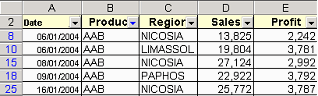
Filtering is a quick way to find a subset of data in a list. There are two filtering methods. The AutoFilter, which was introduced later and is simple to use and the Advanced Filter, which was introduced with the earliest versions of Excel and it's a bit more difficult to use. The illustration below shows an example of AutoFilter where only the records with the "AAB" product are displayed. To do that, select a cell in the Database (click here to download it), select Data /Filter/Autofilter and from the arrow next to the Product field select "AAB". A limitation of AutoFilter is that you can filter the data by only one criterion of the same field (eg either product AAB or ABB etc). If you want to filter by more than one criteria you can use the EasyFilter, a free Add-In developed by Ron de Bruin which can use up to five criteria. You can also use the Advanced Filter method that can cope with even more complex situations.
|
|
|
|
|
|
|
|
|
|
 |
|
|
|
|
|
|
|
|
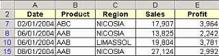
The illustration below shows how the Advanced Filter can be used to display all the records in the region of Nicosia and Limassol, which have the products AAB, ABB, ABC.
|
|
|
|
|
|
|
|
 |
|
|
|
|
|
 |
|
|
|
|
|
|
|
|
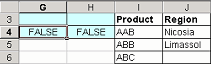
The followings are the steps to do this:
1. Enter the Criteria range as follows:
In G4 enter:
=NOT(ISNA(MATCH($B3,$I$3:$I$6,0)))
In H4 enter:
=NOT(ISNA(MATCH($C3,$J$3:$J$6,0)))
|
|
|
|
|
|
|
|
|
|
 |
|
|
|
|
|
 |
|
|
|
|
|
|
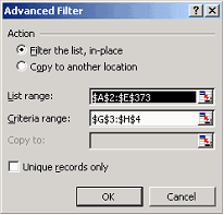
2. Select a cell in the database and chose Data / Filter / Advanced Filter. Complete the window as shown at the right and press OK.
|
|
|
|
|
|
|
|
|
|
|
|
|
|
|
|