Climate
Notes
(last
updated: Dec 27, 2007)
This page contains rough
notes and/or
detailed information about various climate issues, intended to
supplement the web page on the
Science
of Climate Change.
New...
The surface area of the Earth is 510,072,000 km², or 5.1 x 108 x 106 = 5.1 x 10¹⁴ m²
Carbon added by humans to the atmosphere: 100 ppm x 2.1 Gt / ppm x 1012 kg / Gt = 2.1 x 10¹⁴ kg.
Therefore 2.1 x 10¹⁴ kg / 5.1 x 10¹⁴ m² , or 0.4 kg per square meter.
Atmospheric Pressure is 1 kilogram per square centimeter of surface area, or 10,000 kg / m². [ref]
Carbon dioxide has increased by 0.01% of the atmosphere (by volume).
Therefore 0.01% x 10,000 kg / m² = 1 kg / m², but only 1/3 of that is carbon, so we get 0.33 kg / m².
In a study that analyzed temperatures around the globe, researchers
found that Earth has been warming rapidly, nearly 0.36 degrees
Fahrenheit (0.2 degrees Celsius) in the last 30 years... in a
2003 study, scientists showed that 1,700 plant and animal
species migrated toward the poles at about 4 miles per decade in the
last 50 years. That migration rate is not fast enough to keep up with
the current
rate of movement of a given temperature zone, which has reached about
25 miles (40 kilometers) per decade in the period 1975 to 2005, Hanson
and co-authors write in the current issue of the journal Proceedings of
the National
Academy of Sciences
(ref)
In a warm climate, the Hadley cell gets weaker, the cell gets wider,
and the jets and storm tracks penetrate further poleward. This all goes
under the general rubric of "expansion of the tropics," [rc]
Nordhaus Economic Model
If you drive 10,000 miles a year in a car that gets 28 miles per gallon. Your car will emit about 1 ton of carbon per year.
CO2, which has a weight of 3.67 times the weight of carbon.
A typical U.S. household, which uses about 10,000 kilowatt-hour (kWh)
of electricity each year. If this electricity is generated from coal,
this would release about 3 tons of carbon.
For example, if a country wished to impose a carbon tax of $30 per ton
of carbon, this would involve a tax on gasoline of about 9 cents per
gallon. Similarly, the tax on electricity would be
about 1 cent per kWh, or 10 percent of the current retail price, on coal-generated electricity.
|
$100 per ton carbon |
$100 per ton CO2 |
| Added Cost of Gasoline |
$2.50 per liter |
68 cents per liter |
| Added Cost of Electricity |
3.3 cents per kilowatt hour |
0.9 cents per kilowatt hour |
| Annual Emissions |
CO2 Concentration |
Temperature |
Reference |
|
450 ppm |
|
SPM |
|
1000 ppm |
|
SPM |
|
|
|
|
| 19 Gt |
685 ppm |
5.3 |
|
Slide show: 200
million years of Antarctica's drift
Modelling
Climate and
Climate Sensitivity
The equation below illustrates the major factors governing the
temperature of the Earth. The left side describes the
incoming
solar energy and how some is lost to the reflectivity (albedo) of the
planet. The right side is about energy radiated back into
space.
T is the temperature at which the Earth radiates energy,
which
decreases as greenhouse gas levels rise.
| Earth's Energy Balance Equation |
| (S / 4) (1 -
albedo) = σ ε
T4 |
S =
albedo =
σ =
ε =
T = |
Solar
Energy received from the Sun.
Reflectivity of the Earth's surface
the Stefan Boltzmann constant
A measure of how efficiently the Earth dissipates heat
Temperature of the earth-atmosphere system, in °K |
The new best estimate based on the published results for the radiative
forcing due to a doubling of CO2 is 3.7 Wm-2,
which is a reduction of 15% compared to the SAR. The forcing since
pre-industrial times in the SAR was estimated to be 1.56 Wm-2;
this is now altered to 1.46 Wm-2. [IPCC
6.3.1]
The radiative forcing due to CH4
is 0.48 Wm-2 since pre-industrial times (and
0.15 for N2O). [IPCC
6.3.2]
The radiative forcing due to all well-mixed greenhouse gases since
pre-industrial times was estimated to be 2.45 Wm-2
in the SAR with an uncertainty of 15%. This is now altered to a
radiative forcing of 2.43 Wm-2 with an
uncertainty of 10%.
Radiative Forcing of Greenhouse Gases, from [IPCC
Table 6.2]
| Greenhouse Gas |
Simplified Relative
Forcing |
More complex version |
| CO2 |
 F = 5.35 ln(C/C0) F = 5.35 ln(C/C0) |
F= 4.841 ln(C/C0)
+ 0.0906 ( C - C0) C - C0) |
| CH4 |
F = 0.036 (M – M0)
– (f(M,N0) – f(M0,N0)) |
| N2O |
F= 0.12 (N – N0)
– (f(M0,N) – f(M0,N0)) |
f(M,N) = 0.47 ln[1+2.01x10⁻⁵ (MN)0.75+5.31x10⁻¹⁵
M(MN)1.52]
C is CO2
in ppm
M is CH4
in ppb
N is N2O in ppb
The calculated global mean radiative forcing of sulfate aerosol ranges
from -0.26 to -0.82 Wm-2, although most lie in
the range -0.26 to -0.4 Wm-2. Until
differences in estimates of radiative forcing due to sulphate aerosol
can be reconciled, a radiative forcing of -0.4 Wm-2
with a range of -0.2 to -0.8 Wm-2 is retained. [IPCC
6.7.2]
The estimate of the global mean radiative forcing for Black Carbon
aerosols from fossil fuels is revised to +0.2 Wm-2
(from +0.1 Wm-2) with a range +0.1 to +0.4 Wm-2.
[IPCC
6.7.3]
The estimate of the radiative forcing due to biomass burning aerosols
remains at -0.2 Wm-2. The uncertainty
associated with the radiative forcing is very difficult to estimate due
to the limited number of studies available and is estimated as at least
a factor of three, leading to a range of –0.07 to
–0.6 Wm-2. [IPCC
6.7.5]
Therefore a tentative range of -0.6 to +0.4 Wm-2
is adopted for mineral dust; a best estimate cannot be assigned as yet.
E is change in forcing
using the derivative of Stefan-Boltzmann:
dT/dE = 1/(4[sigma] T^3)
dT/dF=1/(4σT3).
gets:
dT=[alpha]ln([CO2]/[CO2}orig)/(4[sigma] T^3)

This is the equation without all feedbacks.

Substituting a doubling CO2 level (unrealistic, according to Lomborg)
and substituting T= 15 degreesC = 288.16K
dT=5.35ln2/(4*5.6705E-08*(288.16^3))
or
dT=0.6833 centigrade for a doubling of CO2 !!

That's physics. All the rest is models and hype.[ref]
Converting Carbon Dioxide Increase into Temperature Change
The direct increase in radiative forcing (dE) caused by an
increase in carbon dioxide levels, in watts per square meter, can be
found by the equation
dE =
5.35 ln (C/Co) W/m2
where C is
the new carbon dioxide level (in parts per million, or ppm) and Co is the
starting carbon dioxide level. For example, CO2
concentration has risen from 270 to 370 ppm, so the
equation gives 5.35 x
ln(370/270) = 1.7 W/m2
raw forcing.
According to the Stefan-Boltzmann equation: Power per unit area (W/m2) =
σ ε
T4
σ =
the Stefan Boltzmann constant, or 5.6703 x 10⁻⁸
Watts / m2 °K
ε
=
A measure of how efficiently the Earth dissipates heat, here assumed to
be 1.
T = Temperature of the earth-atmosphere system, in
°K
Taking the derivative, we get
dT / dE = 1 / ( 4
σ T3
)
Thus
dT =
5.35 ln (C/Co) / ( 4
σ T3
)
T should
be the radiating temperature of the planet, since the
greenhouse effect work because the Earth radiates at a colder
temperature than
the surface. The radiating temperature is about 255K. [But what is the relationship
between the Earth's radiating temperature and the suface temperature?]
| Radiative
Forcing Calculator |
|
|
|
the proof that global warming is anthropogenic is that night and winter
temperatures are rising faster than when the sun is shining. If the
warming was natural then it must be due to the sun. Therefore, day and
summer temperature would show the greatest increase.)
The net amount of solar radiation arriving on
a 1 m 2 area
(perpendicular to sun) on the earth's
surface is S(1- albedo).
From the point of view of the sun, the earth appears to be a
disk
with a radius R, so the total amount of power absorbed by
the whole earth is the product of the arriving solar radiation
times the area of a disk the size of the earth:
PGain = π R2
S(1-alpha)
Any object at a temperature TK (in
Kelvin) will emit
thermal radiation at a rate given by:
PLoss= epsilon σTK4
times it surface area. The factor epsilon
is the emissivity (approximately 1), sigma
is Stefan's constant, and
the total surface area of the spherical earth
(4 π R2).
Recall that a temperature in Kelvin is TK=T0+T
where T is the temperature in centigrade and T0=273.15
In the steady state, the incoming radiation must balance the
outgoing
radiation. This leads to an energy balance equation for
PGain=PLoss:
π R2
S(1-albedo) =
(4 π R2)
σ(T+T0)4
where T is the average temperature of the earth in centigrade.
Solving for T gives the following equation:
T =
[S(1-albedo)/4
/
σ]
1/4-T0.
Where the symbols are defined as:
| T |
The Temperature of the Earth in Centigrade |
| S |
Solar Constant (1370 W/m2)
|
albedo
|
Albedo - Fraction of incident solar radiation reflected
(about 0.32) |
| σ |
Stefan's Constant (5.6696E-8 W/m2K4)
|
| T0 |
Conversion from Kelvin to Centigrade (273.15) |
[ref]
The radiative forcing for CO2
is
roughly proportional to the logarithm 4.4log(C) / log(2)
of its concentration, while for CH4,
the forcing scales like the square root [IPCC, 2001]. This implies that
the higher the base level, the smaller the forcing will be from a fixed
increase in concentration. [ref:
[26]] Using CO2
concentrations of 270 and 540 ppm of , we get 35.5 W/m2
and 39.0 W/m2,
a difference of 4.4 W/m2.
From this NOAA
web page: (also this
overview)
...net planetary
radiative forcing changes roughly linearly
in response to logarithmic changes in CO2.
Thus, a
quadrupling of CO2
gives another roughly 1°C direct
warming over the direct 1°C warming for a CO2
doubling,
valid for the extreme assumption that water vapor mixing ratios and
clouds do not change.
The log-linear relationship
has been found to hold down to CO2 concentrations to as low as
one sixty-fourth of preindustrial
levels. As CO2 is
decreased, the atmosphere's ability to hold water vapor collapses and
the
global temperatures drop sharply. [ref]
A Quick Calculation of Climate Sensitivity for the 20th
Century
We can use the climate forcing figures from the above table, plus the
fact that global average temperature increased by
0.8 ºC, to
calculate the temperature rise for the equivalent of a doubling of
carbon dioxide. The net forcing for the 20th century is 1.6 W/m2.
From this we must subtract the estimated 0.3 W/m2
of energy that has been absorbed by the ocean, thus not included in the
surface temperature (from Lyman et. al.) The forcing from a
full
doubling of CO2
is 3.7 W/m2,
therefore the observed temperature increase is found my multiplying the
temperature increase by the ratio of the present forcing to a
full CO2
doubling:
0.8 ºC * 3.7 W/m2
/ ( 1.6 W/m2
- 0.3 W/m2
) = 2.3 C
This is a bit less than the standard 3 ºC estimate
for a CO2 doubling.
But the uncertainty in these figures is large, so this value fits well
within the range of the IPCC estimates.
From Hansen 2008:
Climate
forcing in the LGM equilibrium state, relative to the Holocene, due to
the slowfeedback ice age surface properties, i.e., increased ice area,
different vegetation distribution, and continental shelf exposure, was
-3.5 ± 1 W/m2 (10). The forcing due to reduced amounts of longlived
GHGs
(CO2, CH4, N2O) was -3 ± 0.5 W/m2, with the indirect effects of CH4 on
tropospheric ozone and stratospheric water vapor included (fig. S1).
The combined 6.5 W/m2 forcing and global surface temperature change of
5 ± 1°C relative to the Holocene (10b,c), yields an empirical
sensitivity ~¾ ± ¼ °C per W/m2 forcing, i.e., a Charney sensitivity of
3 ± 1 °C for the 4 W/m2 forcing of doubled CO2. This empirical
fast-feedback climate sensitivity allows water vapor, clouds, aerosols,
sea ice, and all other fast feedbacks that exist in the real world to
respond naturally to global climate change.
Climate sensitivity
varies as Earth becomes warmer or cooler. Toward colder extremes, as
the area of sea ice grows, the planet approaches runaway snowball-Earth
conditions, and at high temperatures it can approach a runaway
greenhouse effect (8). At its present temperature Earth is on a flat
portion of its fast-feedback climate sensitivity curve.
The
calculation above is for a long period of time and includes all the
slow feedbacks, so I do not know why Hansen calls it a fast feedback.
Since the greenhouse gas portion is about half of the total forcing (ie. 1 + 1 = 2), if
you consider them the cause (or at least the main feedback) then you get a GHG
sensitivity of about 6 degrees. With ice sheets pushing below 45
degrees of latitude, this looks close to a snowball-Earth condition which has a high climate sensitivity.
Luckily the same thing was not also happening in Asia, or we might no be here to write about it. A look at the
<a
href="http://commons.wikimedia.org/wiki/Image:Five_Myr_Climate_Change.png">increasing
temperature response</a> to the same orbital forcings as average
temperature dropped shows that climate sensitivity became significantly
larger during the Pleistocene ice ages.
I am surprised that
Hansen did not use the Pliocene (about 3 million years ago) as a
benchmark. Here we have CO2 levels around 400 ppm, global average
temperature about 2 or 3 degrees higher, and sea levels 25 to 35 meters
higher (think ten storey building). The carbon dioxide forcing is about
the same ( 280 ppm Interglacial / 180 ppm LGM is close to 400 ppm
Pliocene / 280 ppm Interglacial ) for a temperature change about half
as much, implying a much lower climate sensitivity, closer to three
degrees rather than six for the period we are about to enter.
I
still do not think you can use the temperature (or CO2 level) for the
initialitation of glaciation to be the same as that sufficient to melt
the ice cap. For a large continent like Antarctica I think it will take
a few extra degrees to overcome the thermal inertial of all that ice,
unless someone can demonstrate why ths is wrong.
Greenhouse
Effect
Electromagnetic radiation has two properties - wavelength
and intensity.
-------------------
306
http://www.realclimate.org/index.php/archives/2007/05/the-weirdest-millennium/#comment-34515
There are two major effect of changing temperature. The first is to
change the distribution of ground vibrational level quantum states,
which changes the opacity of the system as a function of photon
frequency. The second is to change the thermal distribution of
population in the first excited level of the two degenerate bending
modes, which means that the intensity and frequency distribution of the
emission changes.
309: At low temperature and pressure, there is less opportunity for
molecules to collide with one another (think top of the atmosphere). At
higher pressures and temperatures, the molecules are more likely to
interact, which leads to a broadening of the absorption lines.
291: the absorption per molecule at line center is HIGHER for colder
molecules.
331: But then there is also the blurring of the spectra at higher
pressures.
This is due to the fact that these molecules which are absorbing and
re-emitting radiation are in motion as a result of their temperatures,
colliding and either losing some amount of energy or gaining some
amount of energy prior to absorbtion or re-emission - and as such more
or less energy will be required to enter either the excited or grounded
state.
Visible sunlight penetrates easily through the air and warms the
Earth's surface. When the surface emits invisible heat radiation, some
of it is absorbed by CO2 in
the middle levels of the atmosphere. Thus some energy transfers into
the air itself, rather than escaping directly into space. Not only is
the air thus warmed, but also some of the energy trapped there is
radiated back to the surface, warming it further.
443: Vibrational radiative lifetimes are very long, seconds.
Collisional
lifetimes at atmospheric pressure are of the order of 1-10
microseconds. However, the amount of energy necessare to excite a CO2
bend (~600 cm-1) is about 3x the average energy of a collision at 300 K
(~200 cm-1) so about 5% of all CO2 molecules at 300 K are excited, just
not the same ones at any instant. This is a steady state problem.
458: I don't think absorption of a photon affects the molecule's bond
energy
per se; what it does is kick an electron of one atom in that molecule
to a higher, less stable level. The molecule will then lose energy
either by radiating or by hitting another molecule.
adds 4 Watts per square meter to the planets radiation balance for
doubled CO2.
That's only about a percent of the solar energy absorbed by the Earth,
but it's a highly important percent to us! After all, a mere one
percent change in the 280 Kelvin surface temperature of the Earth is
2.8 Kelvin (which is also 2.8 Celsius).
Re #<a href=""></a>:
Greenhouse Effect References:
- These lecture
notes treat the atmosphere as a constant temperature black
body, and claim a greenhouse effect factor of 1.189 x 255
K = 303 K.
- RealClimate discussion
- Learning from a Simple Model.
- Real
Climate: CO2 colliding with itself in
a tube of pure CO2 broadens the lines about 30%
more than does CO2 colliding with N2
or O2 in air.
- Ray Pierrehumbert in Real Climate - Busy
Week for Water Vapor
- Spencer Weart - Simple
Greenhouse Models and an overview
of the historical development.
- CO2 is cycled through the atmosphere in a period of about
7.5 years. See: http://www.whrc.org/carbon/index.htm
Where it all goes to is not known http://www.whrc.org/carbon/missingc.htm
but much of it gets transported to the deep ocean by the thermohaline
circulation. That is replaced by CO2 that has remained in the deep
ocean for around 1000 years, which is depleted in C14.
- the lapse rate generally increases with altitude in the
troposphere. It
starts out at about 4.75 K/km near ground level and increases to almost
9.8 K/km near the tropopause. The average is around 6.5 K/km.
- Water
vapor at 1% corresponds to about 60% relative humidity at 15 °C [ref]
- Roger Pielke: Relative
Roles of CO2 and Water Vapor in Radiative Forcing + comment:
"...it is clear that the value of 3.7 Watts per square meter for
doubling is not correct."
- GHG
Radiation calculator.
- water vapor is roughly eight times more effective than
carbon dioxide as a greenhouse gas (Hartmann 1994). [nasa]
- Wikipedia
- Most of the infrared absorption in the atmosphere can be thought of
as
occurring while two molecules are colliding. The absorption due to a
photon interacting with a lone molecule is relatively small.
- wiki
- carbon dioxide is a linear molecule, but it has an important
vibrational mode in which the molecule bends with the carbon in the
middle moving one way and the oxygens on the ends moving the other way,
creating some charge separation, a dipole moment,
thus carbon dioxide molecules can absorb IR radiation. Collisions will
immediately transfer this energy to heating the surrounding gas. On the
other hand, other CO2 molecules will be vibrationally excited by
collisions. Roughly 5% of CO2 molecules are vibrationally excited at
room temperature and it is this 5% that radiates.
- http://en.wikipedia.org/wiki/Emission_line
- Science:
The global warming feedback is based on the fact that cold air radiates
less than warm air; if water vapor increases and is distributed to
higher, colder altitudes, less heat is radiated to space and thus
climate warms.
- [ref]
Water
absorbs the Infrared Radiation incoming from Sun because the frequency
of the internal vibration of the water molecules is the same frequency
of the waves of the solar Infrared Radiation. This form of Radiative
Heat transfer is known like Resonance Absorption
Weart:
- The Earth must radiate back into space as much total energy
as it receives, to stay in equilibrium. Adding gas to the atmosphere
moves the site of this emission to higher levels, which are colder.
Cold things radiate less than warm ones, so the system must warm up
until it can radiate enough.
- When the surface emits invisible heat radiation, some of it
is absorbed by CO2 in the
middle levels of the atmosphere. Thus some energy transfers into the
air itself, rather than escaping directly into space. Not only is the
air thus warmed, but also some of the energy trapped there is radiated
back to the surface, warming it further.
Questions:
- Does Kirchhoff's Law apply to a greenhouse gas?
The gas
will absorb radiation at certain frequencies, and radiate at the same
frequencies. It does not act like a black body.
- Is there any validity to the idea that when a greenhouse
gas
molecule
absorbs radiation, this induces vibration which transfers motion, thus
heat, to the surrounding atmosphere? Does this process happen
in
reverse, ie, a collision induces a vibrational state which causes the
GHG to emit a photon?
- Does the Stefan Boltzmann law apply to intensity of
radiation emitted by a greenhouse gas at a certain temperature?
- How much effect is there from atmospheric pressure causing
the absorption spectrum of a greenhouse gas to broaden?
- Can the downwelling longwave radiation be measured at the
surface? Can
we tell from the wavelength which greenhouse gas it came from?
Reference?
The Reflector:
This model recognizes that when a greenhouse
gas absorbs radiation, it re-radiates it in all directions, including
up and down. Greenhouse warming is caused by the portion of longwave
radiation that is returned to the surface. Adding more greenhouse gas
reduces the amount of radiation that is prevented from leaving the
Earth and is instead returned to the surface. More of the greenhouse
effect takes place higher in the atmosphere where the ratio of carbon
dioxide to water vapor is higher, implying that carbon dioxide is a
relatively more important greenhouse gas than in the first model.
The average mass of the atmosphere is about 5,000 trillion
metric tons
or 1/1,200,000 the mass of Earth. According to the National Center for
Atmospheric Research, "The total mean mass of the atmosphere is
5.1480×10¹⁸ kg with an annual range
due to water vapor of 1.2 or 1.5×10¹⁵
kg depending on whether surface pressure or water vapor data are used;
somewhat smaller than the previous estimate. The mean mass of water
vapor is estimated as 1.27×10¹⁶ kg and
the dry air mass as 5.1352 ±0.0003×10¹⁸
kg." [wikipedia]
Table of Greenhouse Gas Forcings
The largest and most certain change in radiative forcing since the
pre-industrial period is an increase of about 2.4 W/m2
due to an increase in well-mixed greenhouse gases (Chapter 6, Figure 6.8 and Table 6.1). Radiative forcing here
is taken to be the net downward radiative flux at the tropopause (see Chapter 6). Smaller, less certain
contributions have come from increases in tropospheric ozone (about
0.3 W/m2),
the direct effect of increases in
sulphate aerosols (about -0.4 W/m2)
and
decreases in stratospheric ozone (about -0.2 W/m2).
[IPCC]
.
| Forcing
Agent |
Forcing
(W/m2)
|
Error |
| Carbon
Dioxide |
1.46 |
| Methane |
0.48 |
| Nitrous
Oxide ( N2O) |
0.15 |
| Halocarbons |
0.35 |
| TOTAL well mixed
greenhouse gases |
+2.43 |
10% |
| Stratospheric O3 |
-0.15
|
67% |
| Tropospheric O3 |
+0.35
|
43% |
| Direct sulphate aerosols |
-0.40
|
200% |
| Direct biomass burning aerosols |
-0.20
|
300% |
| Direct FF aerosols (Black Carbon) |
+0.20
|
200% |
| Direct FF aerosols (Organic Carbon) |
-0.10
|
300% |
| Direct mineral dust aerosols |
-0.60 to +0.40
|
| Indirect aerosol effect {1st
effect only; all aerosols} |
0 to -2.0
|
| Land-use (albedo) |
-0.20
|
100% |
| Solar |
+0.30
|
67% |
| TOTAL |
|
|
...back to main
page
African Climate Change
in 10,000 Years
The vegetation of Africa is compared for 8,000 years ago, during the
mid-Holocene warming when it was
about a degree or two warmer, with today. [ref]
A warmer climate is
clearly a wetter one. Forested areas expand, and climate
zones
shift away from the equator. Note that the Sahara was not a desert at
all (the yellow is grassland, not desert). The temperature
difference is well within the range predicted to occur during the 21st
century due to global warming. Does the map on the left show
what
the consequence will be?
Not right away, at least. The paleoclimate data is from a
climate
in equlibrium, while the near future will be a climate in transition.
There are several reasons while it may take some time to
reach
equilibrium rainfall levels
- The ocean does not warm as quickly as the land.
Moisture
levels are largely determined by sea surface temperature, which lags
behind land temperature. A warmer landmass on its own tends
to
increase the evaporation rate, which could lead to drying.
- Rainfall is also influenced by existing vegetation.
Increased vegetation generates more rainfall, in a positive
feedback loop. But it takes time for vegetation to establish
itself.
Paleoclimate Stuff
[ref] The record obtained
at these sites allowed us to evaluate the causes and effects of several
major global events in Earth history, including:
- Demonstrating
that the latest Cenomanian-Turonian (C/T) ocean anoxic event was
unrelated to sea-level change on million-year or 100-k.y. scales.
- Suggesting
that a major cooling spanning the Campanian/Maastrichtian boundary was
associated with a sea-level lowering and inferred ice volume increase.
- Correlating a latest Maastrichtian global warming with Deccan trap volcanism.
- Linking
the marine mass extinctions at the end of the Cretaceous with ballistic
ejecta. In addition, we showed that collapse of the vertical isotopic
gradient ("Strangelove Oceans") extended to neritic environments and
that there was minimal change in sea level associated with the
Cretaceous/Tertiary (K/T) boundary.
- Establishing that low
 13C and 18O
and high kaolinite values were associated with the Paleocene/Eocene
thermal maximum (PETM) in NJ neritic sections and that isotopic values
remained low and kaolinite remained high throughout a thick section
above the carbon isotope excursion (CIE). This reflects either that
warmer and wetter climate persisted for >300-400 k.y. in NJ (unlike
deep-sea records that show an exponential return to pre-PETM conditions
after ~200 k.y.) or that the extremely rapid deposition of this section
occurred in response to a cometary impact.
13C and 18O
and high kaolinite values were associated with the Paleocene/Eocene
thermal maximum (PETM) in NJ neritic sections and that isotopic values
remained low and kaolinite remained high throughout a thick section
above the carbon isotope excursion (CIE). This reflects either that
warmer and wetter climate persisted for >300-400 k.y. in NJ (unlike
deep-sea records that show an exponential return to pre-PETM conditions
after ~200 k.y.) or that the extremely rapid deposition of this section
occurred in response to a cometary impact.
- Showing
that a large (~60 m), earliest Oligocene drop in sea level was
associated with development of an ice sheet equivalent in size to the
modern East Antarctic ice sheet, though sea level again rose by nearly
50 m ~1 m.y. later, suggesting near collapse of the ice sheet. The ice
sheet subsequently grew and decayed numerous times in the
Oligocene-middle Miocene.
Greenland
Ice Balance
Summing best
estimates of the various mass balance components for Greenland gives a
balance of –8.5 ± 10.2% of the input, or +0.12
± 0.15 mm/yr of global sea level change, not significantly
different from zero. [IPCC
2001] See also IPCC
prediction for the future.
North Atlantic Oscillation
Strong
positive
phases of the NAO tend to be associated with above-averagel
temperatures in the eastern United States and across northern Europe
and below-average temperatures in Greenland and oftentimes across
southern Europe and the Middle East. They are also associated with
above-average precipitation over northern Europe and Scandinavia in
winter, and below-average precipitation over southern and central
Europe. Opposite patterns of temperature and precipitation anomalies
are typically observed during strong negative phases of the NAO. During
particularly prolonged periods dominated by one particular phase of the
NAO, anomalous height and temperature patterns are also often seen
extending well into central Russia and north-central Siberia. [ref]

No positive correlation between arctic SAT and the NAO before 1950 is
found – in fact, here we find that the correlation is
negative (r
~ -0.39). [Nansen]
An Example of Visually Inflating
Climate Data
The figure below shows the change in the melt extent of the Greenland
ice cap between 1992 and 2002. This figure was used in the Arctic
Climate Impact Assessment, by James Hansen in this
paper, and by Al Gore in "An Inconvenient Truth". There are
two reasons it is misleading:
- The concept of "melt extent" does not refer to a net loss
of ice, as one might think. Instead it is defined here
as "experiencing
at least 1 melt day between April 1 - September 25".
This metric is used
because liquid water absorbs energy differently than ice and snow,
making it easy to detect from satellites. So the red area is not
actually melting, it just means it got warm enough for liquid water to
appear at least one day that year.
- The dates 1992 and 2002 have been
chosen (ie. cherrypicked) to select the lowest and highest values on
record. 1992 was the year after the Mount Pinatubo volcanic eruption,
which caused global cooling. The green line on the graph (drawn by me)
shows the rate of increase
presented on the maps, which is many times greater than the actual
average
rate of increase, shown by the red line.

Approximately 98% of the energy supplied annually to the Arctic system
is advected from lower latitudes by the atmosphere [Nakamura and Oort,
1988]. [98% of what?
This can't include the average 100 w/m2
solar
insolation.] Models predict (and observations
seem to confi rm) that warming
is enhanced in the Arctic [Arctic Climate Impact Assessment, 2005].
Consequently, the meridional poleward temperature gradient may decrease
and reduce the northward transport of sensible heat into the Arctic
(heat that is associated with the physical temperature of air parcels).
This negative feedback could slow the transition to the new
state, but a compensating increase in the poleward transport of latent
heat may occur (heat stored as water vapor, which is released upon
condensation). Thus, changes in energy transport from lower latitudes
provide no definite brake on the system.
Arctic cloud cover might also slow the warming: Cloud cover is
decreasing in winter and increasing in other seasons [Wang and Key,
2003]. Over ice-covered areas, however, the shading effect will be
small owing to low surface-cloud contrast in refl ectivity, and thus
additional clouds should enhance longwave emission and warm the surface
[Shupe and Intrieri, 2004]. Therefore, cloud-radiation feedbacks are
not expected to derail the Arctic’s trajectory.
[ref]
If warming stabilises at 3 degrees Celsius, the ice sheet could survive
for several thousand years. But if temperatures rise by 8 degrees
Celsius, which several scenarios predict, then it would disappear in
1000 years.
Advection is the result of extensive cooling, sort of like a thermal
engine where cold and warm air is continuously exchanged, this process
slows down when the Arctic is warmer. The Arctic cools down
substantially depending on how much heat is lost
especially during the long night, it is an ideal location for
determining Global Warming trends because of wider temperature
discrepancies caused by apparently minor (CO2) changes.
Annual mean incoming solar radiation north of the Arctic circle is 100
W/m2, most of it between the spring and autumn
equinoxes.
In summer the energy supply to the arctic climate system is controlled
by absorbed solar radiation, whereas in winter the arctic energy budget
is dominated by advection from lower latitudes.
Antarctica
For Antarctica (Table 11.6), the ice discharge
dominates the uncertainty in the mass balance of the grounded ice
sheet, because of the difficulty of determining the position and
thickness of ice at the grounding line and the need for assumptions
about the vertical distribution of velocity. The figure of Budd and
Smith (1985) of 1,620x1012 kg/yr is the only
available estimate. Comparing this with an average value of recent
accumulation estimates for the grounded ice sheet would suggest a
positive mass balance of around +10% of the total input, equivalent to
-0.5 mm/yr of sea level. [IPCC
2001]
Melting of all existing glaciers and ice caps would raise sea level by
0.5 m (Table 11.3). For 1990 to 2100 in
IS92a, the projected loss from land-ice outside Greenland and
Antarctica is 0.05 to 0.11 m (Table 11.12). [IPCC
2001]
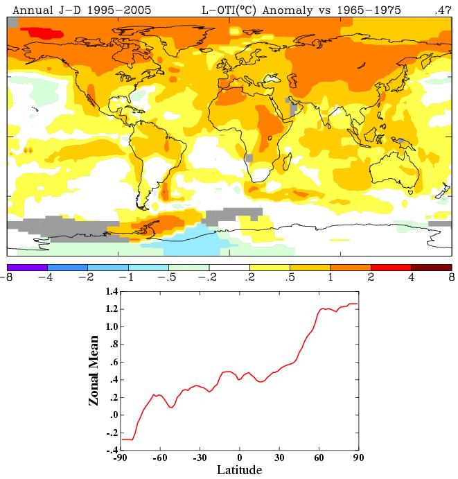
Arctic
Temperature and Sea Ice Changes

Hovmöller diagram indicating the time–latitude
variability
of surface air temperature (SAT) anomalies north of 30°N,
1891-1999: (a) Observed
This image shows the difference between 2005 surface air temperatures
in degrees Celsius (averaged for January through August) and the
fifty-year mean (1955-2004) for the same months. The preponderance of
positive values indicates an unusually warm Arctic in 2005. (NCEP/NCAR
Reanalysis; NOAA-CIRES Climate Diagnostics Center ) [Return
to Press Release]
Arctic
Temperature and Sea
Ice Extent
Satellite data suggest a net decrease in Arctic ice extent of about 2.9
percent per decade. [ref]
The following two graphs are taken from the 2004 Arctic Climate Impact
Assessment paper.
The temperature graph shows a linear rise from 1900 to
1940, a drop from 1940 to 1970, and a rise from 1970 to 2000.
The
slope of both the rise and fall is about the same. The sea
ice
graph shows no change between 1900 and mid century, then what
looks like a linear decline. The decline in summer
starts
around
1950, while the winter decline takes until 1970 to begin.
- Why does the temperature
rise in the early part of the century
have no affect on sea ice extent?
- Why does the decline in
summer sea ice extent begin in 1950,
while the cooling trend does not reverse itself until 1970?
- Why does the caption
attached to the graph suggest the change in
sea ice extent is accelerating? A regression taken from 1900
will
give an exponential curve. But visually at least, the decline
seems to start abruptly, and looks linear after that.


These maps show the difference between
“normal” sea ice extent
(long-term mean), and the year indicated. The long-term average minimum
extent contour (1979-2000) is in magenta. The ice extent for each year
is shown by the edge of the colored region; within that extent, color
bands show differing levels of sea ice concentration. Blue indicates
areas where concentration is more than the long-term mean; red shows
areas where concentration is less than the long-term mean. The 2005 map
shows a marked reduction in extent over the past four years, all of
which were also below average.
In 2002 and 2003, the
ice pack also experienced much lower concentrations during the minimum,
especially true north of Alaska. However, the ice cover has been much
more compact during the minimums of 2004 and 2005, yielding small
negative or even positive ice concentration anomalies within the ice
pack.
Sea Ice extent is a measure of the area that
contains at least 15 percent ice. Ice concentration is the fraction of
the actual area covered by ice compared to the total area, measured in
terms of percentage ice cover. The satellite does not pass directly
over the North Pole; this lack of data is indicated by the gray circle
in each image.
Access 1980
and 2005 images for print and online use.
Ice cap sizes
North America
Ice volume in this subset of tests spans a range of 28.5-38.9 x
10[1][5] m[3] at LGM, with a predominant cluster at 32-36 x 10[1][5]
m[3]. Taking floating ice and displaced continental water into account,
this corresponds to 69-94 m eustatic sea level (msl). More than 75% of
the accepted tests fall in the range 78-88 msl. We argue that this is a
plausible estimate of the volume of water locked up in the NAIS at LGM. [ref]
For our standard run we find a maximum ice volume of 57 × 106 km3
at 18.5 ka cal BP. This corresponds to a eustatic sea level lowering of
110 m after correction for hydro-isostatic displacement and anomalous
ice resulting from defects in the specified boundary conditions of the
Paleoclimate Model Intercomparison Project (PMIP) for which the UKMO
GCM results were generated. Of this 110 m, 82 m was stored in the North
American ice sheet and 25 m in the Eurasian ice sheet. [ref]
Antarctica
At glacial maximum, ice sheets buried almost the entire land surface of
Antarctica and extended across the continental shelf, depositing
sediment on the continental shelf, slope and rise. Sea level was some
120-135 m lower than today, with 12-26 m of this locked up in the
Antarctic ice sheet. Since glacial maximum, the ice sheet has thinned
by hundreds of metres in some areas and retreated inland as much as
1000 km, leaving its imprint on mountain ranges and on the seabed, and
a detailed history in marine sediments. [ref]

[ref]
Paleo Sea Level in the Holocene
The general pattern seems to be sea levels rose to a
maximum of 2 or 3
meters around 5,000 years ago, and gradually declined after that. This
matches the temperature chart for the time period. This water can only
come from
significant melting of the Greenland and/or West Antarctic ice caps.
The missing value is the actual global average temperature, but it
is probably not more than one or two degrees above today, within range
of what global warming can lead to in this century. But unlike today
the temperature changed gradually over thousands of years. So a
tentative conclusion is global warming could lead to ice cap melting,
but we do not know how long it would take. This is much the same
message as from the Eemian interglacial data.
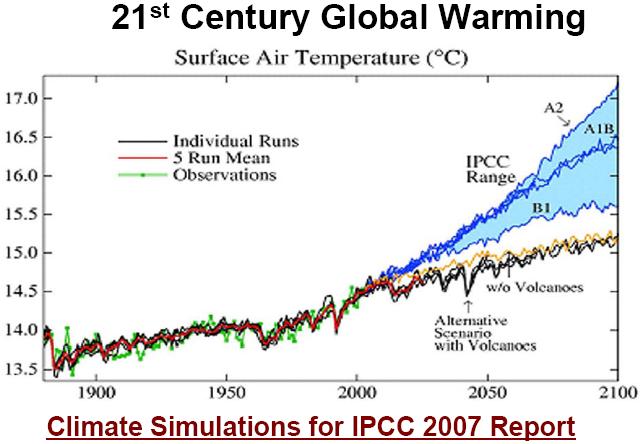
A
Climate Model for the Twentieth Century
Weather forecasts take today’s situation and calculate how it
will
evolve over the next few days. They are initial value problems. Climate
models do not assimilate current data but instead produce changes in
climate as a function of changing boundary conditions, and thus are a
boundary value problem - that is not the same as a forecast (which
would require an estimate of the ‘weather’
component as well as the
climate component). If you know anything about differential equations,
you know those are fundamentally different kinds of problems. [ref]


The four-member ensemble
mean (red
line) and ensemble member range (pink shading) for globally averaged
surface air temperature anomalies (°C; anomalies are formed
by subtracting the 1890–1919 mean for each run from its time
series of annual values) for all forcing [(volcano + solar + GHG +
sulfate + ozone)]; the solid blue line is the ensemble mean and the
light blue shading is the ensemble range for globally averaged
temperature response to natural forcing calculated as a residual
[(volcano + solar)]; the black line is the observations after Folland
et al. (2001). Taken from Meehl et al. (2004).

Smoothed, zonal mean anomalies of surface temperature (in K) for the
observations in each latitude band from 1890-1999. Anomalies are
relative to the 1961-1990 climatology. SOURCE: Delworth and Knutson
(2000).
1940s-1970s cooling is a combination of increasing aerosols, increasing
volcanoes (particularly Mt. Agung in 1963) and a slight decline in
solar forcing, overcoming a relatively slow growth in greenhouse gases.
[ref]
Model simulations for the future are called projections, not
predictions. No-one in this game ever thinks they are predicting the
future, although it often gets translated that way in the popular
press. We take assumptions that people have made for the future and see
what consequences that would
have for the climate.
Why the 1940-1970 cooling? Two abrupt dips, in 1940 and 1960.
Sulphur emissions increased steadily until World War I, then levelled
off, and increased more rapidly in the 1950s, though not as fast as
greenhouse gas emissions. [ref]
Volcanic Eruptions
Major volcanos: None line up with 1940 and 1960.
| Date |
Location |
Lava and Ash |
Aerosol (Sulphur) |
Global Temperature |
| 16 ± 1 My |
Roza flow of the Columbia River Flood Basalt |
|
576 Tg S |
|
| 640 Ky |
Lava Creek Tuff of the Yellowstone Caldera |
1000 km3
lava |
|
|
| 1783 |
Grimsvotn (Laki
or Lakagigar), Iceland |
15.1 km3
lava |
122 Tg SO2 |
-1.3 °C across Euope and N. America |
| 1815 |
Tambora, Sumbawa, Indonesia |
160 km3 ash |
|
|
| 1835 |
Cosiguina, Nicaragua |
|
|
|
| 1875 |
Askja, Iceland |
|
|
|
| 1883 |
Krakatau, Indonesia |
20 km3 ash |
|
|
| 1886 |
Okataina (Tarawera), North Island, New Zealand |
|
|
|
| 1902 |
Santa Maria, Guatemala |
|
|
|
| 1907 |
Ksudach, Kamchatka, Russia |
|
|
|
| 1912 |
Novarupta (Katmai), Alaska, US |
|
|
|
| 1919 |
Kelut Indonesia
|
|
|
|
| 1930 |
Merapi Indonesia |
|
|
|
| 1937 |
Rabaul Caldera Papua New
Guinea |
|
|
|
| 1951 |
Lamington, Papua New Guinea, |
|
|
|
| 1951 |
Hibok-Hibok, Philippines |
|
|
|
| 1963 |
Agung, Bali, Indonesia |
|
|
|
| 1980 |
Mt. St. Helens, Washington, US |
|
|
|
| 1982 |
El Chichòn, Chiapas, Mexico |
2.5 km3 ash |
|
|
| 1985 |
Nevado del Ruiz, Colombia |
|
|
|
| 1991 |
Mt. Pinatubo, Luzon, Philippines |
11 km3 ash |
|
|
from Large
Holocene Eruptions
Natural Forcings (from IPCC)
-3 Wm-2 (for El Chichon and Mt. Pinatubo
eruptions)
WIthout the re-supply of CO2 from geological sources incuding volcanic
degassing, it has been calculated that removal of CO2 from the
atmosphere by silicate weathering, carbonate deposition and the burial
of organic matter could potentially deplete to CO2 content of the
pre-industrial atmosphere in 10,000 years, and the atmosphere-ocean
system in 500,000 years. [ref]
CO2 flux at Marine Ocean Ridges is estimated to be 66 to 97 Mt / year.
This appears to be balanced by the sink provided by
hydrothermal
alteration of newly formed ocean floor lavas.
...return to Paleoclimate
Beginning of a
Simplified Climate Model
CS = Climate Sensitivity = 2.7
CA = carbon content of atmosphere, in ppm
CAR = CO2 increase rate in atmosphere
GE = greenhouse gas emission rate = 1.6%
AA = atmosphere absorption percentage = 0.58%
E = Carbon emission rate
CAR = E * AA
CA(n) = CA(1970) * (1 + rate) ^ years
1970: E = 4 Gt C / yr = 1.9 ppm / yr, CAR = 1.3 ppm
/ yr; CA = 325 ppm; T = 14.0
2005 = E = 7.5 Gt / yr = 3.5 ppm/yr, CAR = 2 ppm /
yr; CA = 375 ppm; T = 14.5
2100 (IPCC B1) T = 15.6
Regional Amplification
Ocean = 0.7
45 deg. N = 1.5
60 deg. N = 2.5
Relationship of
Hurricane Intensity with Global Warming
Other factors being equal, hurricane intensity increases by about 5%
for each degree of increase in sea surface temperature.
...an estimate of a 5%–10% increase in maximum wind speeds
for a
2°C change in SST. The increase in intensity found by WHCC is
equivalent to a 5% increase in maximum wind speeds for a 0.5°C
SST
increase, which is a factor of 2–4 larger than that estimated
from theory and determined from the model simulations of Knutson and
Tuleya (2004). Recent simulations using the Japanese Earth Simulator
(Oouchi et al. 2006) found a 10.7% increase in intensity for a
2.5°C increase in SST, which scales linearly to a 2.1% increase
in
intensity for a 0.5°C increase in SST, which is approximately a
factor of 2 smaller than the increase found by WHCC. [Ref]
The observed SST increases in
the Atlantic and Pacific tropical cyclogenesis
regions range from 0.32°C to 0.67°C
over the 20th century. [ref]
The temperature gradient that matters for hurricanes is the difference
between the sea surface and the top of the troposphere, and if the
vertical structure breaks down due to wind shear the hurricane
dissipates or won't form.
Mid Latitude Storms
The factors that control this are often confounding and so make this a
tricky prediction. Simple arguments based on the expected 'polar
amplification'
and the fact that the surface temperature gradient between the tropics
and the poles will likely decrease would reduce the scope for
'baroclinic instability' (the main generator of mid-latitudes storms).
However, there are also increases in the upper
troposphere/lower stratospheric gradients (due to the stratosphere
cooling
and the troposphere warming) and that has been shown to lead to
increases in wind speeds at the surface. And finally, although latent
heat release (from condensing water vapour) is not a fundamental driver
of mid-latitude storms, it does play a role and that is likely to
increase the intensity of the storms since there is generally more
water vapour available in warmer world. It should also be clear that
for any one locality, a shift in the storm tracks (associated with
phenomena like the NAO
or the sea ice edge) will often be more of an issue than the overall
change in storm statistics. [RealClimate]
Solar
Driven Climate Change
The Solar constant above Earth's atmosphere is 1368 W/m2 ±
0.1%, possibly related
to sunspots. But most of that radiation reaches the Earth's
surface obliquely, and half of the Earth is in darkness. The mean solar
energy reaching the Earth's surface is 265 W/m2.
- These satellite instruments suggest a variation in annual
mean TSI of
the order 0.08% (or about 1.1 W/m2)
between minimum and maximum of the 11-year solar cycle. [IPCC
6.11]
- Solar irradiance change has a strong spectral dependence
[Lean, 2000],
and resulting climate changes may include indirect effects of induced
ozone change [RFCR; Haigh, 1999; Shindell et al., 1999a] and
conceivably even cosmic ray effects on clouds [Dickinson, 1975].
Furthermore, it has been suggested that an important mechanism for
solar influence on climate is via dynamical effects on the Arctic
Oscillation [Shindell et al., 2001, 2003b]. [ref]
- Time-dependent experiments produce a global mean warming of
0.2 to
0.5°C in response to the estimated 0.7 W/m2
change of solar radiative forcing from the Maunder Minimum to the
present. (from IPCC
2001). But,
from IPCC 2007: Changes in solar irradiance since 1750 are
estimated to cause a radiative forcing of +0.12 [+0.06 to
+0.30] W/m2,
which is less than half the estimate given in IPCC 2001.
- A U.S. National Academy of Sciences panel estimated that if
solar
radiation were now to weaken as much as it had during the 17th-century
Maunder Minimum, the effect would be offset by only two decades of
accumulation of greenhouse gases. As one expert explained, the Little
Ice Age "was a mere 'blip' compared with expected future climatic
change." [ref]
- A half of a percent change in solar output could raise
temperatures,
eventually [over a century], about three-quarters of a degree Celsius,
which,
coincidentally, roughly equals the observed warming in the past
century,” says Hansen. [ref]
Solar Forcing
Since 1600 (from Lean
and Rind, 1998)

Compared are
decadally average values of the Lean et
al. (1995b) reconstructed solar total irradiance (diamonds) from Fig.
13 and NH summer temperature anomalies from 1610 to the present. The
solid line is
the Bradley and Jones (1993) NH summer surface temperature
reconstruction from paleoclimate data (primarily tree rings), scaled to
match the NH instrumental data (Houghton et al. 1992) (dashed line)
during the overlap period.
Galactic Cosmic Radiation
From [ref]
The GCR flux incident on Earth’s atmosphere is modulated by
three processes:
a) variations of the solar wind within the heliosphere (on
10–1000 yr timescales, and possibly longer)
b) variations of Earth’s magnetic field (100–10,000
yr)
c) variations of the interstellar flux outside the heliosphere
(>10 Myr).
On reaching Earth, cosmic rays must traverse the geomagnetic field to
reach the lower atmosphere. In consequence, the GCR intensity is about
a factor 4 higher at the poles than at the equator, and there is a more
marked solar cycle variation at higher latitudes.
The GCR flux over these different timescales varies by between 15%
during the 11 yr solar cycle, to as much as a factor 2 increase during
periods of low geomagnetic field and low solar activity. Interstellar
modulations of the GCR flux are estimated to be between -75% and +35%
of present values [28] on cosmological timescales, corresponding to the
140 Myr crossing period of the solar system with the spiral arms of the
MilkyWay (where the peak fluxes probably reside). Nearby supernovae
could increase the GCR fluxes above these values. In summary, if the
cosmic ray-climate connection is causal, then the climate appears to be
remarkably sensitive to quite small secular changes of GCR
intensity—of around 10% or so.
[How can] an energetically-weak GCR signal (which is roughly equivalent
to that of starlight) is amplified into a significant climate forcing.
Distribution of
Energy Use
Environment Canada - Canada Office of Energy Efficiency
Canada’s GHG
Emissions by Sector, End-Use and Sub-Sector
– Including
Electricity-Related Emissions
| |
2004 |
| Total
GHG
Emissions Including
Electricity (Mt of CO2e) |
|
505.4 |
| |
| Residential
(Mt of CO2e) |
|
76.7 |
| Space
Heating |
|
41.3 |
| Water
Heating |
|
19.2 |
| Appliances |
|
11.5 |
| Major
Appliances |
|
7.0 |
| Other
Appliances |
|
4.5 |
| Lighting |
|
4.0 |
| Space
Cooling |
|
0.8 |
| |
| Commercial/Institutional
(Mt of CO2e) |
|
67.9 |
| Space
Heating |
|
34.1 |
| Water
Heating |
|
5.7 |
| Auxiliary
Equipment |
|
10.2 |
| Auxiliary
Motors |
|
6.0 |
| Lighting |
|
7.1 |
| Space
Cooling |
|
4.2 |
| Street
Lighting |
|
0.5 |
| |
| Industrial
(Mt of CO2e) |
|
169.7 |
| Mining |
|
37.8 |
| Pulp
and Paper |
|
23.4 |
| Iron
and Steel |
|
17.7 |
| Smelting
and Refining |
|
15.5 |
| Cement |
|
4.7 |
| Chemicals |
|
10.6 |
| Petroleum
Refining |
|
22.3 |
| Other
Manufacturing |
|
31.6 |
| Forestry |
|
1.8 |
| Construction |
|
4.1 |
| |
| Total
Transportation (Mt of CO2e) |
|
176.4 |
| |
| Passenger
Transportation (Mt of CO2e) |
|
94.3 |
| Cars |
|
43.8 |
| Light
Trucks |
|
30.1 |
| Motorcycles |
|
0.2 |
| Buses |
|
3.6 |
| Air |
|
16.5 |
| Rail |
|
0.2 |
| |
| Freight
Transportation (Mt of CO2e) |
|
75.4 |
|
Light Trucks |
|
12.8 |
|
Medium Trucks |
|
10.3 |
|
Heavy Trucks |
|
36.8 |
| Air |
|
1.1 |
| Rail |
|
5.8 |
|
Marine |
|
8.7 |
| |
| Off-Road
(Mt of CO2e) d,e |
|
6.6 |
| |
| Agriculture
(Mt of CO2e) a,e |
|
14.7 |
One barrel of oil (42 U.S. gallons, or 159 liters) can provide about 6
million Btu.
CO2 released per barrel of oil (distillate fuel)= 0.47 tons, or 0.003 tons / liter
So a carbon tax of $30/ton CO2 is about 10 cents per litre.
$30 / ton CO2 = 7.25 cents per litre [ref]
$37 per ton of carbon "starter tax" mentioned earlier, equating to around 10 cents a gallon of gasoline
8.8 kg CO2/ US Gal. [ref]
times 1 gal / 3.785 liters
2.3 kg CO2 / litre
US CO2 emissions
21% Residential - 12% light 40% heat and cool
18% commercial - 20% light 18% heat and cool
28% Industrial
A typical new 1000-MW coal-fired power station produces around 6
million tons of carbon dioxide annually.
The carbon content of natural gas is only 60
percent that of coal per unit of primary energy content.
"When the ‘best guess’
estimates of radiative forcing are applied to global average coal and
gas characteristics, the benefits of fuel switching are delayed by
about 30 years," Jain said. "The delay is caused by the reduction in
sulfate aerosol emissions and increase in natural gas-related methane
emissions that occurs when switching from coal to natural gas
– creating a net warming effect." [ref]
However, coal and gas use also release methane, the second most
important greenhouse gas emitted by human activities. During coal
extraction, methane trapped in and around coal seams is released to the
atmosphere. Methane also is released whenever natural gas escapes
during transportation and distribution. Hence, switching from coal to
gas would reduce methane emissions from coal mining, but increase
natural gas-related emissions.
Mountain
Pine Beetle
Beetles and Cold Weather
[ref]
- Cold weather kills the mountain pine beetle. Mountain pine
beetle eggs, pupae and young larve are the most susceptible to freezing
temperatures.
- In the winter, temperatures must consistently be below -35
Celsius or -40 Celsius for several straight days to kill off large
portions of mountain pine beetle populations.
- In the early fall or late spring, sustained temperatures of
-25 Celsius can freeze mountain pine beetle populations to death.
- A sudden cold snap is more lethal in the fall, before the
mountain pine beetles are able to build up their natural anti-freeze
(glycerol) levels.
- Cold weather is also more effective before it snows. A deep
layer of snow on the ground can help insulate mountain pine beetles in
the lower part of the tree against outside temperatures.
- Wind chill affects mountain pine beetles, but is usually
not sustained long enough to significantly increase winter mortality.
Historical
Mountain Pine Beetle Activity
Mountain pine beetle (MPB) has been present in British Columbia's
forests for millenia. Foresters have recorded MPB outbreaks in some
parts of BC since 1910. However, evidence of MPB activity going back
hundreds of years is found in scars on lodgepole pine trees.
Impacts
of Climate Change on Range Expansion by the Mountain Pine Beetle
Abstract: The current latitudinal and elevational range of mountain pine beetle
(MPB) is not limited by available hosts. Instead, its potential to
expand north and east has been restricted by climatic conditions
unfavorable for brood development. We combined a model of the impact of
climatic conditions on the establishment and persistence of MPB
populations with a spatially explicit, climate-driven simulation tool.
Historic weather records were used to produce maps of the distribution
of past climatically suitable habitats for MPB in British Columbia.
Overlays of annual MPB occurrence on these maps were used to determine
if the beetle has expanded its range in recent years due to changing
climate. An examination of the distribution of climatically suitable
habitats in 10-year increments derived from climate normals (1921-1950
to 1971-2000) clearly shows an increase in the range of benign
habitats. Furthermore, an increase (at an increasing rate) in the
number of infestations since 1970 in formerly climatically unsuitable
habitats indicates that MPB populations have expanded into these new
areas.
The potential for additional range expansion by MPB under
continued global warming was assessed from projections derived from the
CGCM1 global circulation model and a conservative forcing scenario
equivalent to a doubling of CO2 (relative to the 1980s) by
approximately 2050. Predicted weather conditions were combined with the
climatic suitability model to examine the distribution of benign
habitats from 1981-2010 to 1941-2070 for all of Canada. The area of
climatically suitable habitats is anticipated to continue to increase
within the historic range of MPB. Moreover, much of the boreal forest
will become climatically available to the beetle in the near future.
Since jack pine is a viable host for MPB and a major component of the
boreal forest, continued eastward expansion by MPB is probable.
Justice Michael Burton on Al Gore's "An Inconvenient Truth"
[from here]
Untruth 1
Gore says: A sea-level rise of up to seven metres
will be caused by melting of either West Antarctic or Greenland ice cap
in the near future. Cities such as Beijing, Calcutta and Manhattan
would be devastated.
Judge says: "This is distinctly alarmist,
and part of Mr. Gore's 'wake-up call.' It is common ground that if
indeed Greenland melted, it would release this amount of water, but
only after, and over, millennia, so that the Armageddon scenario he
predicts, insofar as it suggests that sea-level rises of seven metres
might occur in the immediate future, is not in line with the scientific
consensus."
Untruth 2
Gore says: Low lying inhabited
Pacific atolls are being inundated because of anthropogenic global
warming. "That's why the citizens of these Pacific nations have all had
to evacuate to New Zealand."
Judge says: "There is no evidence of any such evacuation having yet happened."
Untruth 3
Gore says: The shutting down of the "Ocean Conveyor" would lead to another ice age.
Judge says: "According to the Intergovernmental Panel on Climate
Change, it is very unlikely that the Ocean Conveyor (an ocean current
known technically as the Meridional Overturning Circulation or
thermohaline circulation) will shut down in the future, though it is
considered likely that thermohaline circulation may slow down."
Untruth 4
Gore
says: Two graphs relating to a period of 650,000 years, one showing
rise in CO2 and one showing rise in temperature, show an exact fit.
Judge
says: "Although there is general scientific agreement that there is a
connection, the two graphs do not establish what Mr. Gore asserts."
Untruth 5
Gore says: The disappearance of snow on Mt. Kilimanjaro is expressly attributable to global warming.
Judge
says: "The scientific consensus is that it cannot be established that
the recession of snows on Mt. Kilimanjaro is mainly attributable to
human-induced climate change."
Untruth 6
Gore says: The drying up of Lake Chad is a prime example of a catastrophic result of global warming.
Judge says: "It is generally accepted that the evidence remains insufficient to establish such an attribution."
Untruth 7
Gore says: Hurricane Katrina and the consequent devastation in New Orleans is due to global warming.
Judge says: "It is common ground that there is insufficient evidence to show that."
Untruth 8
Gore says: Polar bears have drowned swimming long distances to find ice.
Judge
says: "The only scientific study that either side before me can find is
one which indicates that four polar bears have recently been found
drowned because of a storm."
Untruth 9
Gore says: Coral reefs are bleaching because of global warming.
Judge
says: "The actual scientific view, as recorded in the IPCC report, is
that, if the temperature were to rise by 1-3 degrees centigrade, there
would be increased coral bleaching and widespread coral mortality,
unless corals could adapt or acclimatize."
Two more, from Real Climate
At one point Gore claims that you can see the aerosol concentrations
in Antarctic ice cores change "in just two years", due to the U.S.
Clean Air Act. You can't see dust and aerosols at all in Antarctic
cores — not with the naked eye — and I'm skeptical you can definitively
point to the influence of the Clean Air Act.
Another complaint is the juxtaposition of an
image relating to CO2 emissions and an image illustrating invasive
plant species. This is misleading; the problem of invasive species is
predominantly due to land use change and importation, not to "global
warming".
See also Misleading Statistics on Greenland
Infall of Extraterrestrial
Material to Earth
About 40,000 tons of extraterrestrial matter, ranging from sub-micron
size dust up to objects tens of meters in size, accretes onto the Earth
each year. We estimate that, in the current era interplanetary dust
contributes
~15 tons/year of unpyrolized organic matter to the surface of the
Earth. During the first 0.6 billion years of Earth's history, this
contribution is likely to have been much greater.
Roughly
500 meteorites larger than 0.5
kilograms are thought to fall on Earth every year (reference).
1000 kg of Martian material falls to Earth each year. 500
kg of Martian rocks larger than 100 mm
fall to Earth each year.
Return
to the Climate Change Main Page

 13C and

