4
Experimental Results
4.1 Image Capture
The Experiment conducted, consisted of taking stereo images at certain
intervals, and then tracks the robots movements. The robot was instructed
to move forward 100 cms. each time. Measurements were taken (see Table
1), and the robots odometry readings noted (see Table 2).
Table 1. Robots location experimentally
measured in the laboratory.
|
Location
|
Location (x,y,z)
|
dx
|
dz
|
|
0
|
257.5
|
0
|
0
|
|
|
|
1
|
257.5
|
0
|
100
|
0.0
|
100
|
|
2
|
264.0
|
0
|
199
|
6.5
|
99
|
|
3
|
269.5
|
0
|
298
|
5.5
|
99
|
|
4
|
275.5
|
0
|
400
|
6.0
|
102
|
Table 2. Robots location obtained by its
own odometry.
|
Location
|
q (degrees) |
x (cms.) |
z (cms.) |
dx |
dz |
Distance to front wall |
|
0
|
0.00
|
0
|
0.1
|
|
|
721.5
|
|
1
|
359.47
|
7
|
98.5
|
7
|
98.4
|
623.1
|
|
2
|
359.16
|
18
|
196.8
|
11
|
98.3
|
524.8
|
|
3
|
358.80
|
34
|
295.0
|
16
|
98.2
|
426.6
|
|
4
|
358.48
|
59
|
398.4
|
25
|
103.4
|
323.2
|
To begin, the images captured are chromatic, but dont need this much
information, so only the blue component con the images is stored. The images
are also reduced to one quarter to improve speed in detecting features.
The resulting images are achromatic (grey scale) and occupy 384´
288 pixels, see Figure 7.
Figure 7. Stereo
images captured at initial position.
4.2 Feature Detection
Once the images were stored we attempt to find 25 features in each image.
The KLT filter to find features is constrained by the following parameters:
|
Parameter
|
Value
|
| mindist |
20
|
| window_size |
7
|
| min_eigenvalue |
1
|
| min_determinant |
0.01
|
| min_displacement |
0.1
|
| max_iterations |
10
|
| max_residue |
10
|
| grad_sigma |
1
|
| smooth_sigma_fact |
0.1
|
| pyramid_sigma_fact |
0.9
|
| sequentialMode |
FALSE
|
| smoothBeforeSelecting |
TRUE
|
| writeInternalImages |
FALSE
|
| search_range |
15
|
| nSkippedPixels |
0
|
Two images are saved Lfeat0.ppm and Rfeat0.ppm showing all the features
detected in each image.
Figure 8. Lfeat0.ppm
and Rfeat0.ppm showing the features detected by the KLT algorithm.
Next the features coordinates xL,yL and
xR,yR
are converted to camera pixels
u = xscale ´ x
v = yscale ´ y
where xscale and yscale are the ratios of the images height
and width respectively.
xscale = 752 ¸ 384
= 1.9583
yscale = 582 ¸ 288
= 2.0208
4.3 Stereo Match

Then for each feature an epipolar line in the right image is calculated
and the nearest features searched in a range given by mindisp=20 and closest
to a predicted disparity given by:
where Z was the approximate distance of the features and B the inter-ocular
separation of the head, 25.2 cms. (see Figure 4).
After all the matches have been found, a search is done to remove any
duplicates, i.e. if two left features are matched to the same right feature.
Now we can calculate the matched features 3D position using the following
head parameters:
Fku = 1939.53;
Fkv = 2009.64;
U0 = 752/2;
V0 = 582/2;
Pp = 25.2/2; /* Horizontal offset
between pan and elevation axes */
Cc = 4.0; /* Offset between elevation
axis and optic axes */
Nn = 7.5; /* Offset along optic axis
between vergence axes and optic
centres of cameras */
Ii = 25.2; /* Inter-ocular separation
*/
Hh =79; /* Height of head centre
above the ground */
And the coordinates, changed to the Fixed World Coordinate Frame. With
this the position of the robot can be estimated and then the appropriate
files are saved (see Figure 9). In file LMatches0.txt the coordinates of
each feature are shown as well as the number of the corresponding feature
in the right image. Features with no match found are given a value of 1.
RMatches0.txt contains the features found in the right image. A value of
1 represents that it has been matched with a left feature, while 1 represents
that no match was found.
File RealWorld0.txt contains the 3D coordinates of the matched features,
as seen in Figure 11.
(a) (b)
Figure 9. (a)
Contents of file LMatches0.txt . (b) Contents of file RMatches0.txt.
The matched features are also placed on the images and saved in PPM
format. Two files are generated; LMatch0.ppm and RMatch0.ppm, see Figure
10. Comparing the image pair in Figure 8 and Figure 10, we see not all
features detected were stereo matched.
Figure 10. Lmatch0.ppm
and Rmatch0.ppm showing matched features in each image.
Figure 11. Contents
of file RealWordl0.txt
4.4 Feature Tracking
At this moments we proceed to track the features from the previous left
image to the new left image taken at the new location. If some features
are not tracked to the next image, the algorithm attempts to find new features
to replace them. Then 25 features are searched in the new right image,
and the process repeats itself.
At the end, a new file is saved containing the history of the features
in the left image, see Figure 12.
Figure 12. Feature
Table showing the feature history in the left side.
In Figure 12, we see that in frame0 (initial location), 16 features
are stereo matched, denoted by their positive values. In frame 1, tracked
features are given a value of zero. Only 5 features are tracked from the
first image to the second. But since the algorithm searched new features
to replace the untracked, in frame 2 we are able to track 8 features. Then
only 2 features were tracked to frame 3, and finally only 1 features is
tracked to frame 4.
4.5 Experimental Environment
The laboratory wall in front of the robot during this experiment is
shown in Figure 13. The robot was placed approximately at 7 mts. from this
wall and then moved toward the wall at 100 cms. intervals. The dimensions
of this wall are shown in Figure 14. And Figure 15, shows the coordinates
of the principal features. The origin for these coordinates was placed
at the bottom-left hand corner of the wall. In Figure 16 the side- wall
is shown with its dimensions.
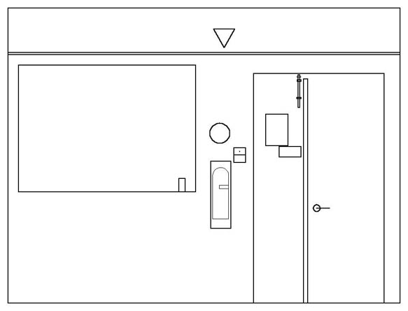
Figure 13. Laboratory
wall which the robot faced during this experiment.
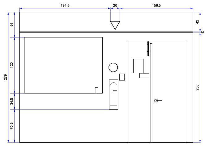
Figure 14. Front
wall with all dimensions shown in centimeters.
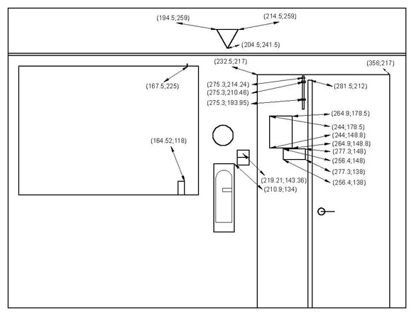
Figure 15. Front
Wall with principal feature coordinates shown.
Figure 16.
Partial view of the side-wall located to the right of the front wall shown
in Figure 13.
4.6
Results
In Table 3 we see the 3D position of some features found at the starting
position. The average error in the x direction is 0.3 cms. In the
vertical direction the average error is 9 cms.
Table 3. Experimental and Real coordinates
of the features matched and found in Figure 15
|
Experimental
|
Real
|
|
|
|
Feature
|
x
|
y
|
z
|
x
|
y
|
dx |
dy |
|
0
|
210.1712
|
124.4368
|
733.8098
|
210.9
|
134.0
|
-0.7
|
-9.6
|
|
2
|
198.1255
|
252.3184
|
707.7735
|
194.5
|
259.0
|
3.6
|
-6.7
|
|
3
|
213.7301
|
252.5516
|
708.869
|
214.5
|
259.0
|
-0.8
|
-6.4
|
|
4
|
281.4418
|
190.4332
|
655.2688
|
281.5
|
212.0
|
-0.1
|
-21.6
|
|
5
|
277.3173
|
142.9643
|
724.0054
|
277.3
|
148.0
|
0.0
|
-5.0
|
|
6
|
245.7721
|
169.7695
|
739.1494
|
244.0
|
178.5
|
1.8
|
-8.7
|
|
8
|
277.4464
|
126.1343
|
720.4741
|
277.3
|
138.0
|
0.1
|
-11.9
|
|
9
|
264.5356
|
167.4504
|
719.7704
|
264.9
|
178.5
|
-0.4
|
-11.0
|
|
11
|
232.0163
|
209.9571
|
753.4997
|
232.5
|
217.0
|
-0.5
|
-7.0
|
|
13
|
277.4094
|
185.1026
|
730.7184
|
275.3
|
194.0
|
2.1
|
-8.8
|
|
14
|
205.1867
|
238.3834
|
710.5756
|
204.5
|
241.5
|
0.7
|
-3.1
|
|
15
|
354.0995
|
208.4073
|
747.6114
|
356.0
|
217.0
|
-1.9
|
-8.6
|
In Figure 18, Figure 19, Figure 20, and Figure 21 the 3D position calculated
for the matched features are shown for each stage. As can be seen the features
appear shifted to the left as the robot progresses. This indicates that
the robot has moved in the positive direction of the x-axis, agreeing with
the robots odometry.
Figure 17. Image sequence of left images
captured during the experiment.
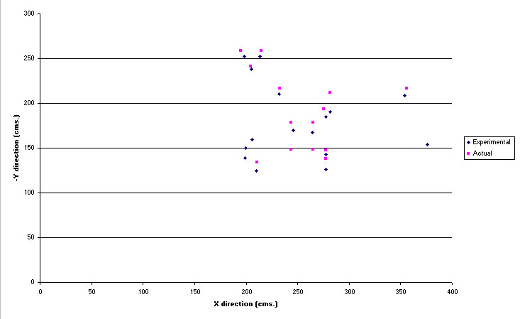
Figure 18. Position
of the features found and actual position of the features shown in Figure
15 at Location 0.
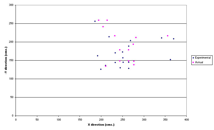
Figure 19. Position of the features found and
actual position of the features shown in Figure 15 at Location 1.
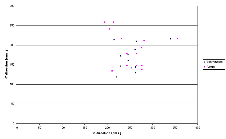
Figure 20. Position
of the features found and actual position of the features shown in Figure
15 at Location 2.

Figure 21. Position of the features found and
actual position of the features shown in Figure 15 at Location 3.
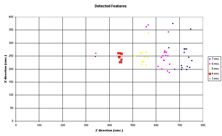
Figure 22. Features detected and stereo matched at each location. The values
used for Z are referenced to the robots coordinate frame.
The results of robot localization are as follow:
|
Location
|
x
|
-y
|
z
|
|
1
|
12.8073
|
-1.2278
|
95.7116
|
|
2
|
3.0721
|
-3.5914
|
90.4321
|
These values show the robot displacement calculated at the given location.
Table 4. Statistics
of Results
| Location |
Features
Found and/or
Replaced |
Matched
Features |
Tracked
Features |
Features used
to Estimate
Position |
|
0
|
22,25
|
16
|
|
|
|
1
|
25,23
|
18
|
5
|
4
|
|
2
|
25,16
|
12
|
8
|
5
|
|
3
|
25,08
|
9
|
2
|
-
|
|
4
|
|
4
|
1
|
-
|
Homepage
| Table of Contents
This page hosted by  Get your own Free Home Page
Last update: 12/11/99
Comments, suggestions and queries to manuel@earthling.net.
Copyright © 1999 Manuel Noriega.

