As seen in Table 3, the current camera calibration gives a pretty good value for the features, although as the robot gets closer, the error in the height increases. The distance to the features is acceptable, and can be seen in the files RealWorldi.txt and given the robot’s distance to the front wall shown in Table 2. The inaccuracy of the cameras is probably due to the fact that the cameras were not accurately calibrated.

Attempting to re-calibrate the cameras, 16 features in the stereo pair obtained at the starting position were used to try to find the fundamental matrix. The 16 features and their coordinates in camera pixels are shown in Table 5. The 8-point algorithm described in [4] was used generating the 16 ´ 9 matrix shown in Table 6. This matrix M is called the measurement matrix. The equation Mf = 0 was solved where f is the fundamental matrix represented as a 9-vector. The solution was f = 0, which is the trivial solution. And therefore could not be used.



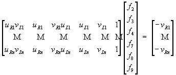
Then a 6-point algorithm was tried, using the value in Table 6 to fill the following equation:

Solving the previous equation gave the following results:
 
 

f2 =	0.002698
f3 =	-0.799357
f4 =	-0.002669
f7 =	0.821643
f8 =	-0.866264
f9 =	-50.599253



These values are part of the fundamental matrix, denoted as the common elevation fundamental matrix.



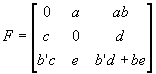
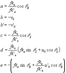
In terms of the camera parameters we have:
 
 

where



(1)
Table 5. Features used to calibrate cameras.
 

xL	yL	xR	yR	uL	vL	uR	vR
100	243	73	246	195.8300	491.0544	142.9559	497.1168
82	60	55	64	160.5806	121.2480	107.7065	129.3312
104	60	77	64	203.6632	121.2480	150.7891	129.3312
199	135	168	136	389.7017	272.8080	328.9944	274.8288
193	215	166	220	377.9519	434.4720	325.0778	444.5760
150	180	124	185	293.7450	363.7440	242.8292	373.8480
193	238	166	244	377.9519	480.9504	325.0778	493.0752
175	180	148	185	342.7025	363.7440	289.8284	373.8480
84	223	57	226	164.4972	450.6384	111.6231	456.7008
133	129	108	134	260.4539	260.6832	211.4964	270.7872
193	157	167	163	377.9519	317.2656	327.0361	329.3904
92	80	65	84	180.1636	161.6640	127.2895	169.7472
296	129	271	135	579.6568	260.6832	530.6993	272.8080
96	194	71	201	187.9968	392.0352	139.0393	406.1808
341	191	312	198	667.7803	385.9728	610.9896	400.1184
76	198	48	206	148.8308	400.1184	93.9984	416.2848

Table 6. 16 ´ 9 measurement matrix.
 

uR*uL	uR*vL	uR	vR*uL	vR*vL	vR	uL	vL
27995.0539	70199.1237	142.9559	97350.3829	244111.3920	497.1168	195.8300	491.0544	1
17295.5744	13059.1977	107.7065	20768.0817	15681.1493	129.3312	160.5806	121.2480	1
30710.1906	18282.8768	150.7891	26340.0061	15681.1493	129.3312	203.6632	121.2480	1
128209.6770	89752.3043	328.9944	107101.2506	74975.4953	274.8288	389.7017	272.8080	1
122863.7722	141237.2019	325.0778	168028.3439	193155.8239	444.5760	377.9519	434.4720	1
71329.8634	88327.6645	242.8292	109815.9808	135984.9669	373.8480	293.7450	363.7440	1
122863.7722	156346.2979	325.0778	186358.7087	237144.7147	493.0752	377.9519	480.9504	1
99324.9173	105423.3415	289.8284	128118.6442	135984.9669	373.8480	342.7025	363.7440	1
18361.6874	50301.6552	111.6231	75126.0028	205806.9178	456.7008	164.4972	450.6384	1
55085.0622	55133.5583	211.4964	70527.5823	70589.6738	270.7872	260.4539	260.6832	1
123603.9154	103757.3045	327.0361	124493.7275	104504.2429	329.3904	377.9519	317.2656	1
22932.9346	20578.1297	127.2895	30582.2666	27442.0113	169.7472	180.1636	161.6640	1
307623.4580	138344.3918	530.6993	158135.0123	71116.4624	272.8080	579.6568	260.6832	1
26138.9435	54508.2998	139.0393	76360.6906	159237.1712	406.1808	187.9968	392.0352	1
408006.8184	235825.3667	610.9896	267191.1852	154434.8192	400.1184	667.7803	385.9728	1
13989.8571	37610.4894	93.9984	61955.9998	166563.2081	416.2848	148.8308	400.1184	1


 

Solving equations (1) we obtain:
 
 

a =	0.002698
b =	-296.256711
c =	-0.002669
d =	0.998117
e =	-0.866264
b' =	-307.815301

And this in turn gives us the following results:
 

qL =	89.845405
qR =	90.152938
v0 =	296.256711
v’0 =	307.815301
fku =	121.497168

which do are not reliable compared to the previous values used. Fk_u has a value that is too small. And when tested gave incorrect results. But since we are only interested in determining the robot’s position from its starting point, we need only be able to determine the robot’s relative movements from its initial location and not the absolute values. Therefore we can use the current camera calibration since relative measurements are mostly independent of camera calibration. And the current calibration is good enough.

The location of the robot could not be calculated at all locations. The only values obtained are for locations 0 through 2. This was due to the fact that not all tracked features could be stereo matched. The algorithms to track features and stereo match are independent and therefore do not guarantee that all tracked features will be stereo matched. In addition, the tracking algorithm only works with the left images and therefore does not know if the feature is no longer visible in the right image.

The algorithm to stereo match features works pretty good, but as seen in Table 4, the KLT tracking algorithm did not find many features even though through careful examination of the features stored in the images, we can see that more features are still visible but were not tracked. This could be due to a great shift in features location from one set of images to the next. Snapshots taken at smaller intervals could provide better results, since features would shift a smaller distance. And more features tracked would provide a better estimate of the robot’s position. Consequently in Figure 23 only the two first legs of the robots journey is displayed. But approximating the location of the robot by averaging all stereo matched features, gives us the results shown in Figure 24. This is only an approximation that is reasonable since most features found are on the front wall and therefore practically at the same distance from the robot in the z-direction. Thus only paying attention on the z-values, we see in Figure 24, that the movement in such direction is pretty well tracked.



Figure 23. Robot progress as detected by vision and odometry.
 
 




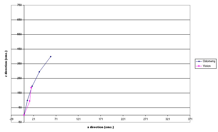
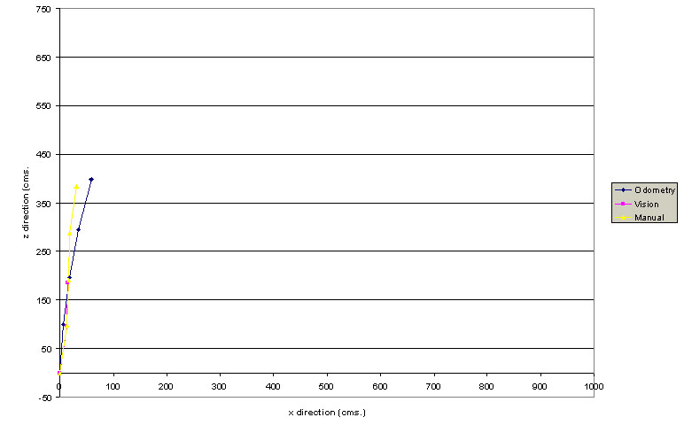
Figure 24. Robot progress including manual calculation of all locations
 
 

We have shown that robot localization is possible even without calibrated cameras, although camera calibration would definitely improve the results. The localization would also improve if more featured could be tracked from one image to the next. This could be achieved by taking snapshots at smaller intervals.

1. A.J. Davison and D.W. Murray, ‘Mobile Robot Localization Using Active Vision’, University of Oxford.
2. Bruce D. Lucas and Takeo Kanade, ‘An Iterative Image Registration Technique with an Application to Stereo Vision’, International Joint Conference on Artificial Intelligence, pages 674-679, 1981.
3. Carlo Tomasi and Takeo Kanade, ‘Detection and Tracking of Point Features’, Carnegie Mellon University Technical Report CMU-CS-91-132, April 1991.
4. F. Li, J. Brady and C. Wiles, ‘Calibrating The Camera Intrinsic Parameters For Epipolar Geometry Computation’, September 1995.
5. Jianbo Shi and Carlo Tomasi, ‘Good Features to Track’, IEEE Conference on Computer Vision and Pattern Recognition, pages 593-600, 1994.
6. K. Onoguchi, M. Watabe, Y. Okamoto, Y. Kuno and H. Asada, ‘A Visual Navigation System using a multi-information Local Map’, 1990 IEEE International Conference on Robotics and Automation, pp. 767-747, 1990.
7. N. Ayache, Artificial Vision for Mobile Robots: Stereo Vision and Multisensory Perception, MIT Press, Cambridge MA, 1991.
8. R. Sim, Mobile Robot Localization Using Learned Landmarks, McGill University, July 1998.
9. S. Kagami, M. Inaba and H. Inoue, The World Map Generation by the Real World Landmark and the Efficient Utilization of it, 12th Robot Symposium, No. 1, pp. 405-406, 1994.
10. Stan Birchfield, Derivation of Kanade-Lucas-Tomasi Tracking Equation, Unpublished, May 1996.
11. T. Kanbara, J. Miura and Y. Shirai, Selection of efficient Landmarks for an Autonomous Vehicle, IROS’93, vol. 2, pp. 1332-1338, 1993.

Homepage | Table of Contents

This page hosted by  Get your own Free Home Page
 

Last update: 12/11/99

Comments, suggestions and queries to manuel@earthling.net.

Copyright © 1999 Manuel Noriega.