Chapter 1   Introduction

 
In repeated measures studies each subject is observed at several different times or under different experimental conditions. Data from such studies have been frequently encountered and analyses of such data are playing an increasingly important role in medical and biological researches, as well as in sociology, economics, education, psychology and other fields (Wrigley, 1986).

Particularly in biomedical sciences, the studies of growth curve, normative aging, chronic diseases, health effect of air pollution, and many other circumstances often involve repeated measures. A typical scenario is that response to a treatment is measured several times during or after its administration, the intention being to compare treatments with respect to the trends in their effects over time as well as with respect to their mean levels of response.

The data from repeated measures is frequently incomplete. Data can be either missing or censored for reasons that are either related or unrelated to the outcome of interest and for reasons that are either planned or accidental. Missing data are one form of incomplete data which contains no information at all. Censored data are another form in which there is only partial information about the measured value. For instance, the data would have been outside a specified range.

The dataset below suffers from this problem. The presence of numerous missing and censored data is the motivation for this dissertation. Beyond this starting point, a systematic approach for a broad class of models with incomplete data is pursued, especially for the general mixed models with multivariate normal distribution.

 
1.1   Motivating Data

Many carcinogens, including the Polycyclic Aromatic Hydrocarbons (PAH), exert their effects by binding to DNA and forming adducts that may lead to mutation and ultimately to cancer. Thus using adducts as biomarkers has the theoretical advantage that they reflect chemical-specific genetic damage that is mechanistically relevant to carcinogenesis (Perera, 2000).

The dataset is from a smoking cessation study of the Molecular Epidemiology Program at Columbia University. Serial samples from 40 heavy smokers (≥1 pack per day for ≥1 year) were tested to validate PAH-DNA adducts as smoking-related biomarkers. PAH-DNA adducts in white blood cells were measured by competitive ELISA (Santella et al., 1990). Subjects were sampled at enrollment while actively smoking. Subjects were brought to measure PAH-DNA at five time points, 10 weeks, then 8, 14, 20 and 26 months (i.e. every 6 months after the 10th week) after quitting. Only successful quitters (≤25 ng/ml for ≥8 months) are included in this study. Quitting was assessed by cotinine, an internal dosimeter of exposure to tobacco smoke.

A significant reduction in PAH-DNA adducts was observed following cessation in all persons who were cotinine-verified quitters. PAH-DNA adducts were significantly higher in persons with the CYP1A1 MspI polymorphism after adjustment for the effect of genotype GSTM1. In prior lung cancer studies, these genetic markers have been associated with increased risk of lung cancer. It is expected that PAH-DNA adducts can be useful as intermediate biomarker in intervention programs and in identifying persons who may be at increased risk of cancer from exposure to cigarette smoke due to high levels of carcinogen binding. For further data description and background information, see Mooney et al. (1995).

There are 40 subjects with 6 measures per subject. All the 240 measures are almost evenly distributed in three categories: complete, censored and missing.

Table 1.1: Measurement Availability for PAH-DNA Over Time
	base line	week 10	month 6	month 12	month 18	month 24	total
censored	13	14	21	11	10	6	75
missing	0	9	5	15	24	28	81
complete	27	17	14	14	6	6	84

Most missing data are due to lost to follow-up, insufficient DNA, destroyed sample, nonfunctioning assay, or the subject was unsuccessful at quitting smoking at some late time point and had to be excluded thereafter. The censored observations (almost 1/3 in this dataset) are due to the ELISA method in laboratory. Briefly, the measurement for a given sample is read off a standard curve. The standard curve is usually not entirely linear, but only the linear portion is used. Subjects with measurements below the linear portion were designated non-detectable (i.e. censored), while others were considered positive. See Santella et al. (1990) for more details about ELISA method. The detection cutoff in this dataset is about 2 adducts per 10⁸ nucleotides, so the censored measure here has a value somewhere between 0 and 2.

This dataset is incomplete and unbalanced, as often seen in longitudinal studies. Some of such characteristics include unequal lengths of follow-up, missing observations, and unequal spacing of measurements over time. As shown in Table1.1, there are a large portion of censored measures, and in fact only 35% measures are accurately available. Table1.2 below gives a closer examination of the data patterns.

Table 1.2: Data Patterns for PAH-DNA Repeated Measures Over Time
baseline	10 week	6 month	12 month	18 month	24 month	count
*	*	*	*	*	0	1
*	*	*	0	0	0	4
*	*	0	0	0	0	1
*	*	1	*	0	0	1
*	0	*	*	*	*	1
*	0	*	1	0	0	1
*	0	1	1	0	1	1
*	1	*	1	0	0	1
*	1	*	1	1	*	1
*	1	1	0	1	1	1
1	*	*	*	0	0	1
1	*	*	0	0	0	1
1	*	*	1	*	*	1
1	*	*	1	0	0	1
1	*	0	*	*	*	1
1	*	0	*	1	1	1
1	*	1	1	*	1	1
1	0	*	*	*	0	1
1	0	*	1	0	0	1
1	0	0	*	*	1	1
1	0	1	0	0	0	2
1	0	1	1	1	1	1
1	1	*	*	*	0	1
1	1	*	*	0	0	2
1	1	*	0	0	0	2
1	1	*	1	1	0	1
1	1	0	1	1	*	1
1	1	1	0	0	0	4
1	1	1	1	*	*	1
1	1	1	1	*	0	1
1	1	1	1	0	0	1
Legend:	1 = complete measurement available 0 = totally missing * = censored/undetectable, but within the range of [0,2).

There are many methods available to handle repeated measurement data with missing outcomes. Other methods are available to handle univariate censored data. However, there are limited methodologies to handle both missing and censoring in repeated measures model and Mixed models in general. Some of these relevant researches will be reviewed in section 1.4, now we briefly examine some problems in commonly used naive methods.

 
1.2   Naïve Method and Problems

When there are censored observations in the data, for example, value given as a subset in the sample space, some analysts treat these values just as other general missing values and exclude them from analysis. This is not plausible as those information contained in the censored data are totally lost, and thus introduces bias in the results.

However, a fairly common practice is to replace those censored observations by the mid-points of the given ranges, or some other values based on distributional or other justifications, before proceed for further analysis. Despite that this might be a better practice than simply throwing away information as one did above, we also should try hard to avoid making up nonexistent “new information”. The fact is, no matter what justification is used for choosing that magic substitution value, at least the following two problems are potentially outstanding.

1.2.1   Distributional Problems

The distribution will be distorted, the extent of which is likely proportional to the percentage of censored observations. This is because a heavy mass was put on that single value, which would spread over the range if they were completely available. For the motivating example above, the distribution of baseline measurement after substituting the censored observation by its midpoint 1 is shown in Figure 1.1. The first bar alone accounts for 13 censored subjects, which would be spread over the range from 0 to 2 if they were available.

Figure 1.1: Distributions after Censored Observations Replaced by Midpoints
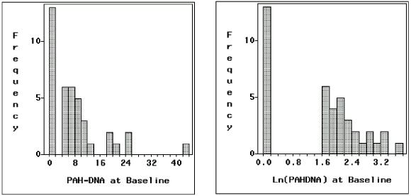(Mean=8.34   Std=8.78   N=40)	(Mean=1.55   Std=1.18   N=40)

1.2.2   Error in Variance Estimation

The naïve variance estimate treats mid-point imputed values as observed, while they are in fact left censored as in this dataset. If we group all subjects into two groups according to their measurements either censored or complete, we have:

Total SS =SS between+ SS within completed + SS within censored.

Now by this value substitution, the last term SS within censored group is 0, which is usually not correct and reduces the variance estimation. This causes the data artificially tight. On the other hand, the first term SS between will be modified in either directions (increase or decrease). Then variance estimation will contain errors, either underestimated or overestimated. For a simple example of inflating variance, consider sample {1, 2, 3} and its replacement {1, 1, 3}. Thus the effect of such substitution on variance estimation is unpredictable.

1.2.3   Monte-Carlo Simulation

As shown in Figure 1.1 log-transformation does not improve the distribution much. Instead, based on the distribution shown in Figure 1.1, we may assume a Gamma distribution and conduct the following Monte-Carlo simulations for the baseline data.

The density function for Gamma distribution with parameters α and β is

if y > 0, and 0 elsewhere.

Its mean is given by αβ and variance by αβ².

In the data, there are 13 censored subjects out of 40 subjects, or about 32.5%. We adjust the parameters α and β to match this censoring percentage in the simulation. The censorship cut point is set to 2, the same value as in the PAH-DNA data set.

In the simulation, we run 1000 samples and each sample has 40 observations independently drawn from the Gamma distribution above. The mean and standard deviation are calculated from both full data (without censoring) and imputed data after replacing left censored data (if less than 2) by the mid-point 1. The results are shown in Table1.3, where the last row Observed %Incomplete is the average proportion of incomplete observations simulated in each sample. To see the effects under various circumstances, we repeat the process with three different settings on α and β.

Table 1.3: Monte-Carlo Simulation: Mean and Standard Deviation Estimation
Mean ± Std Dev	Gamma Distribution Parameters (α, β)
	α=0.5, β=22.8	α=1, β=5.1	α=10, β=0.24
Full data	11.29 ± 15.37	5.07 ± 4.95	2.41 ± 0.76
Imputed data	11.40 ± 15.28	5.09 ± 4.93	2.21 ± 0.97
Theoretical values	11.40 ± 16.12	5.10 ± 5.10	2.40 ± 0.76
Observed %Incomplete	32.5%	32.5%	32.2%

Both the full and imputed statistics yield pretty close estimations for both mean and standard deviation, except in the last column, where the mid-point imputation over-estimates standard deviation. The standard deviations in the first two columns are slightly under-estimated from the imputation. The reason is that the cut point 2 is quite far away from the means in these two settings. As we move the underlying mean downwards to the cut-point, the error in variance estimation could be very severe. This point is illustrated in Figure 1.2, which is obtained by running each simulation with 1000 samples of size 100. We fix α=1 and change β only, so that underlying mean and standard deviation are equal to β. The cut-point is still set to 2. The y-axis %Under Estimation is calculated as the percentage of under-estimation of standard deviation in imputation compared to the original. Both the original sample and its imputed data have under-estimated the true variance in the simulation.

Figure 1.2: Monte-Carlo Simulation of Variance Under Estimation (%)

 
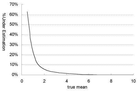1.3   Overview of Proposed Approach

Repeated measures study is very important in contemporary researches. However, it is especially challenging to get complete dataset from such study. Since naive approaches could mislead analysis, new advanced methods are needed to deal with repeated measures while fully taking the data incompleteness into account.

Repeated measures model could be formatted within the framework of the Mixed models. There have been extensive researches in these areas. Many existing results are sound and invaluable, and playing essential role in today's numerous researches. However, many of them handle data with only missing outcomes, but not data with both missing outcomes and censored outcomes simultaneously. Clearly this is due to the significant complexities introduced by censoring. Also most of these results were for multivariate normal distribution, which limited its application as well. Therefore, it would be worthwhile to develop methods that could handle repeated measures with any type of incomplete data and regardless of its distribution. All information available in the data should be effectively utilized as much as possible. This kind of method is increasingly in demand as modern researches advance rapidly.

1.3.1   Approach and Method

At current stage, our approach is fully parametric likelihood. It is conceptually straightforward but computationally challenging. EM algorithm is used to maximize the likelihood, and Monte Carlo Markov chains are generated via Gibbs sampler to implement these algorithms in practice.

In order to handle various models in a uniform fashion, we will first formulate EM algorithm for more general and broader class of models, then show details for special cases within that framework. For example, develop EM algorithm for general model with any distribution, then for exponential family, and then for normal distribution.

Likewise, in order to uniformly handle all kinds of data, either completely known, partially known, or missing, we will treat complete and missing as two extreme cases of incomplete. That is, everything is incomplete in a sense. Missing data is a valid observation with range as large as the whole sample space, e.g. (-∞, +∞) in R¹, and complete data has range of a single point, e.g. [y, y]. In practice, a continuous variable will necessarily be measured actually to only finitely many decimal places. An observed value will therefore correspond to some small interval of real values, say y (y-ε, y+ε). This simple notational convention will enable us to approach all data points in a coherent manner.

The complexity in calculating multi-dimensional integrals was prohibitive for exploiting such approaches as ours in the past. Due to this very reason, many researches were directed on trying to circumvent such calculations and instead to use one dimensional integrals whenever possible. Those attempts are proven useful, but applicable only under some special circumstances. On the other hand, as the computing power has been improving rapidly in recent years, these integral calculations are no longer that overwhelming as it seems. As shown in Chapter 7 by the simulations and real data examples, such calculations are becoming more and more affordable today.

1.3.2   Summary

In current dissertation, we attempt to set up a systematic approach for a broad class of models with censored or missing measures. Specifically, we attempt to extend the conventional analyses in the following aspects:

1. to uniformly handle various types of incomplete data such as missing, right, left, or interval censoring. In fact, data could be in the form of any subset in the sample space;

2. to uniformly handle arbitrary variance-covariance structure and mean-variance structures. By specifying two related Jacobian matrices (4.10), we are able to estimate whatever parameters of interest in a consistent approach;

3. to handle non-normal outcomes, especially from exponential families;

4. to develop an efficient method to approach complex multi-dimensional integrals involved in maximizing related likelihood functions.

As a direction for future development, it is of great interest to generalize the Hierarchical GLM model (Lee & Nelder, 1996) to handle incomplete data with any distribution. HGLM is a class of mixed model arising from exponential family outcomes. Its extension can be easily put into our general framework in Chapter 3.

 
1.4   Review of Some Relevant Researches

The classical linear model has only one error term with normal distribution. There are rich methodological developments and applications based on this well known model.

One of extensions was to linear models for a vector of outcomes. One significant extension in this direction leads to the random effect models and the mixed models, where correlation among the elements in a vector can be induced by sharing random components. In these models, the linear predictor is allowed to have, in addition to the usual fixed effects, one or more random components with assumed distribution. A major extension of linear models to other direction was to the Generalized Linear Models (Nelder & Wedderburn, 1972; McCullagh & Nelder, 1989). In GLM, the class of distributions is expanded from normal distribution to that of exponential families. By introducing the concept of link function, the additivity of systematic effects could occur on a monotonic transformation of the mean, rather than the mean itself. The combination of the prior two extensions produces a class of Generalized Linear Mixed Models (GLMM), and Hierarchical Generalized Linear Models (HGLM) (Lee & Nelder, 1996). The HGLM is further reviewed in section 1.5.1.

Another important development is on yet another different direction. That is to allow outcomes to be incomplete (censoring, truncation or missing). Although the need for methods dealing with such data has long been recognized, the development of proper models has proceeded very slowly due to the difficulties added by incompleteness. For univariate linear models, various extensions of the classical least squares estimators to the censored data have been suggested in the literature (Miller, 1976; Buckley & James, 1979; Koul et al., 1981), notably the Buckley-James estimator. For repeated measures with censored data in mixed models, Pettitt (1986) provided an approach using the EM algorithm, which focused on normal distribution only, see a brief review in section 1.4.2 below.

The Buckley-James method is a non-parametric approach to censored univariate data. For the robustness of non-parametric or semi-parametric methods, it is of great interest to extend the Buckley-James method to handle censored multivariate data. Two such attempts are reviewed in section 1.5.2, namely the marginal independence approach (Lee et al., 1993) and linear mixed effect model approach (Pan & Louis, 2000). Both approaches are applied to the accelerated failure times (AFT) models wherein the failure times are dependent.

1.4.1   Simple Linear Regression with Censored Data

Consider the linear regression model

yi = xi β + εi

(i = 1, ..., n)

(1.1)

where ε_i are independently and identically distributed with unspecified distribution function F, mean zero and finite variance. Suppose that the responses y_i are not completely observable and that the observations are (z_i , δ_i , x_i), where

z_i = min ( y_i , c_i),      δ_i = I ( y_i ≤ c_i)

and (c_i , x_i) are independent random vectors that are independent of ε_i. This is the so called censored regression model with censoring variables c_i.

Various extensions of classical least squares estimators to this censored regression model have been studied (Miller, 1976; Buckley & James, 1979; Koul et al., 1981). Based on some simulation and empirical studies, Miller and Halpern (1982) compared the performances of several such estimators, as well as with the proportional hazards model (Cox, 1972). They concluded that the Cox and the Buckley-James estimators are the two most reliable regression estimates to use with censored data and the choice between them should depend on the appropriateness of the proportional hazards model or the linear model for the data. Heller and Simonoff (1990) have also compared several methods based on an extensive simulation study, they also concluded that the estimator of Buckley-James method is preferred.

Buckley-James Estimating Equation

Buckley-James estimator (Buckley & James, 1979) is an iterative estimator based on the Kaplan-Meier product limit estimate (Kaplan & Meier, 1958) of distribution function F. It provides substitutes for the censored values, and then applies ordinary least squares to the complete set of data.

When the y_i are completely observable, the least squares estimate b_n of β is the solution b=b_n of the normal equation

where . In the case of censored data (z_i , δ_i , x_i) with nonrandom x_i and c_i, Buckley and James proposed to modify the normal equation above as

(1.2)

Noting that . It substitutes an estimate for the conditional expectation based on the Kaplan-Meier estimator into and then solve the usual least squares normal equation iteratively.

Specifically, replace censored values by the conditional expectation , which can be estimated from the Kaplan-Meier estimator. Note that

So it can be estimated by as

(1.3)

where is the Kaplan-Meier estimate of F based on . Then

(1.4)

Thus, the Buckley-James estimator is defined by the equation

(1.5)

This can be solved iteratively as usual least squares normal equation. To start, it seems sensible to take for the starting the least squares estimator

which treats all the observations as uncensored. Then the k+1 step is the usual least squares estimator

The iteration is continued until converges to a limiting value or become trapped in a loop. When it fails to converge and eventually oscillates, one can take the average of the oscillating iterates as the solution (Miller & Halpern, 1982).

In spirit this is a non-parametric version of the EM algorithm introduced by Dempster et al. (1977). The censored observations are replaced by their expectations and then the sum of squares is minimized.

The asymptotic theory for Buckley-James estimator is quite difficult to obtain. The estimator for the covariance matrix of recommended by Buckley and James does not have firm theoretical foundation, but its validity has been empirically substantiated through Monte Carlo simulations. However, with slight modification to the estimator, Lai and Ying (1991) have shown that the estimator is consistent and asymptotically normal.

1.4.2   Repeated Measures with Censored Data

For censored data in mixed effects models, Pettitt (1986) provided an approach using the EM algorithm to get maximum likelihood estimations. The approach was applied to a mixed model for repeated measures with normal errors.

The central part of the approach is to carry out the E-step in a two-stage process, while proceed the M-step as usual. Let Y be the dependent vector. The first stage of the E-step is the regular conditional expectation given Y = y and the parameters of interest, as if there were no censoring on Y at all. The second stage is expectation on the result of the first stage with respect to Y, conditioning on the event of censoring on Y if appropriate, and its marginal distribution.

Now we will go through the general implementation of this EM algorithm in more details for pure random effects model with right censored data as given in the paper.

Let the unobserved q_i×1 vector x_i (i = 1, ..., k+1) be normally distributed with zero mean and covariance matrix times the identity matrix, and let A_i be N × q_i design matrix, so that the observed N × 1 vector Y is modeled as

Y = A x,

with . For the dependent vector Y with possible right censored observations, assume Y_j > y_j if Y_j is censored and Y_j = y_j if y_j is uncensored. Let D be the covariance matrix of x, then Y is marginally distributed with zero mean and covariance matrix

For the usual random effects mode, take and A_k+1 = I, the N × N identity matrix, so that the N × 1 vector x_k+1 is the vector of observation errors.

For the E-step, in the first stage, assume there were no censoring. We require expectations of the with respect to the conditional distribution of x given Y = y and the parameters, which is normal with mean b = DA^TV ^-1y and covariance matrix B = D - DA^TV ^-1AD. Thus we have the marginal mean of x_i given y as b_i, and marginal covariance matrix as B_i. The required expectation is therefore + tr(B_i). Note that the first term involves the y vector as a quadratic from y^TC_i y, the second term tr(B_i) does not involve the y vector.

In the second stage, under normal distribution, since all terms involving y are in the quadratic form y^TC_i y, the only effect of this stage is to replace the term y_j y_k in y^TC_i y by y_jE(Y_k) if y_j is uncensored and y_k is censored, and by E(Y_j Y_k) if both y_j and y_k are censored; if y_j, y_k are uncensored they remain unchanged.

The expectations are with respect to the observed data and marginal distribution of the vector Y = (Y₁, ..., Y_n)^T. Let ƒ(y) be a multivariate normal density with zero mean and covariance V, and let U and C denote the sets of indices of uncensored and censored observations respectively. Then for censored y_k,

To obtain E(Y_j Y_k) for j,k C, replace y_k by y_j y_k above.

The next iteration is then found from as the M-step.

Besides the general result for this pure random effects model with censored data, Pettitt's paper also gave explicit results for the random effects model where random effects are uncorrelated to each other.

 
1.5   Researches Important to Future Development

1.5.1   Hierarchical Generalized Linear Models

The Hierarchical Generalized Linear Model (HGLM) (Lee & Nelder, 1996) is an important methodological advance for analysis of complete data. Its extension to handle incomplete data would be logical next step for future research.

HGLMs allow extra error components in the linear predictors of generalized linear models (GLM). The distributions of these components could be arbitrary. Lee and Nelder (1996) give some HGLM examples for distributions of the Poisson-gamma, binomial-beta and gamma-inverse gamma. The linear mixed models are a special class of HGLM with normal-normal distribution and identity link.

In order to avoid the integration that is necessary when marginal likelihood is used directly, Lee and Nelder used a generalized Henderson's joint likelihood (h-likelihood) for inference from HGLM. Under appropriate conditions maximizing the h-likelihood gives fixed effect estimators that are asymptotically equivalent to those obtained from the use of marginal likelihood; at the same time, obtains the random effect estimates that are asymptotically best unbiased predictors. Important to note, the procedures make no use of marginal likelihood and so involve no complex integrations.

1.5.2   Buckley-James Method and Multivariate Data

In many studies, non-parametric or semi-parametric approaches are preferred for robustness. Therefore it is of great interest to extend the Buckley-James method (Buckley & James, 1979) to handle censored multivariate data.

The Buckley-James method is non-parametric since the distribution function is given by the Kaplan-Meier estimate (Kaplan & Meier, 1958). However, it is very difficult to generalize the Kaplan-Meier method to estimate multivariate distribution function. Consequently, attention is given to the direct use of the univariate Buckley-James method but with appropriate adjustments in modeling or inference. Two such approaches reviewed here are the marginal independence approach and linear mixed effect model approach. Both approaches are aimed at the accelerated failure times (AFT) models wherein the failure times are dependent.

The marginal independence approach (Lee et al., 1993) is to ignore the dependence among multivariate components in estimating the regression coefficients and then appropriately draw statistical inference. Specifically, in the Buckle-James estimating equation (1.5), replace the censored values by estimates given by equation (1.3) as usual. However, the dependence among multivariate components is ignored when estimating the underlying distribution by Kaplan-Meier estimate (1.4), and treated as if from univariate data. Lee et al. (1993) pointed out that this simple approach do have large sample justification. They also examined these properties with some practical sample sizes.

However, ignoring the dependence generally does not take full advantage of the information in the data and is thus not efficient. In the mixed effect model (Pan & Louis, 2000), it is attempt to include a random effect to account for the dependence.

Specifically, for i = 1, ..., n and j=1, ..., n_i, suppose T_ij is (logarithm of) failure times and C_ij is a censoring random variable independent of T_ij. We observe T_ij^* = min (T_ij , C_ij) and δ_ij = I (T_ij ≤ C_ij), where I(.) is the indicator function. The linear mixed effect model is

T_ij = X_ij β + Z_ij b_i + ε_ij ,

where X_ij are covariates, and β is the unknown regression coefficient of primary interest. b_i is the random effect causing the possible correlation among T_ij's for j =1, ..., n_i, and Z_ij =1 is assumed in the article. The mean-zero error ε_ij are now assumed to be independent and identically distributed with distribution function F.

As in the usual linear regression or Buckley-James estimation, the least-squares estimation equation is derived under the assumption ε_ijN (0, σ²). However, when imputing censored data, the distribution function F of ε_ij is estimated by the non-parametric Kaplan-Meier estimate. For b_i, assume that b_iN (0, τ²), also b_i and ε_ij are independent.

The implementation of the estimation procedure is complex. It is based on using Monte Carlo Expectation Maximization (MCEM) to estimate β (Tanner, 1996), and using restricted maximum likelihood (REML) to estimate the variance components τ² and σ² (Diggle et al., 1993). Specifically, denote the matrix notations corresponding to T_ij , Y_ij , X_ij , Z_ij , b_i by T, Y, X, Z, b respectively, the algorithm is as follows:

0. Let be an initial estimate.
1. For k =1 to K (the sample size of Monte Carlo simulation):
   0. Let β ^(k) = .
   1. Generate b^(k) from conditional distribution of b|(T^*, δ).
   2. Impute T from T^* by , where the expectation uses the Kaplan-Meier estimate of distribution of ε_ij.
   3. Let β ^(k) =(X'X) ^-1X' (T ^(k) - Z b^(k)).
   4. Return to step 1.2 until convergence to get the estimate of β ^(k).
2. Let .
3. Impute T from T^* by , using the Kaplan-Meier estimate of the distribution function of ε_ij.
4. Compute the REML estimates (, ), and hence the estimated covariance of T, , using imputed Y.
5. Readjust .
6. Go to step 1 until convergence.

As with the Buckley-James method, the “convergence” in steps (1.4) and (6) implies either a true convergence or that a fixed number of iterations has been reached. The inner loop (steps 1.2-1.4) is not necessary, but may speed up the convergence of the time-consuming outer loop. Step (5) is optional and may improve efficiency when the distribution of Zb + ε is close to a normal.

With censored data, we do not have a closed form estimation for the conditional distribution function in step (1.1). However, the conditional distribution of b_i|(T_i^*, δ_i) is proportional to

where ƒ and g are the normal densities for ε_ij and b_i, respectively, and F is the cumulative distribution function for ε_ij with current estimates of (β, τ, σ) as their parameters. Hence, the Metropolis-Hastings algorithm (Carlin & Louis, 1995) can be used to generate a sample from b_i|(T_i^*, δ_i) with current estimates of (β, τ, σ). It is computationally intensive.

This approach is essentially semi-parametric because of the non-parametric least squares estimation and the Kaplan-Meier estimator. The estimation of τ and σ is parametric as their asymptotic validity depends on the normality assumption. However, these estimates are not used directly in drawing statistical inferences about β. Rather, bootstrap methods are used in numerical example in estimating the standard error of . Simulations show that this approach may be favorable in the multivariate AFT model when compared to the marginal independence approach, especially when the correlation is strong among failure times.