Chapter 7   Data Simulation and Example

 
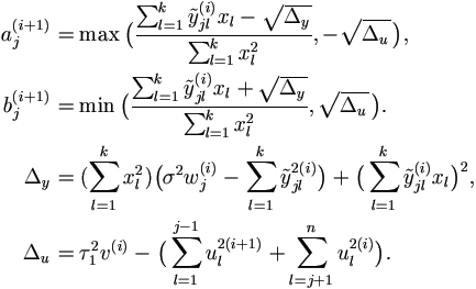
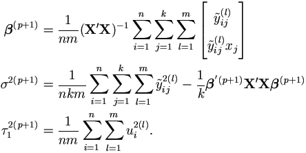
In this Chapter, we apply the Gibbs sampler in Theorem 6.3 to implement the MCEM algorithm outlined in Theorem 4.5. First, a Monte Carlo simulation is performed as an example of using the MCEM algorithm and to assess its performance. Second, the motivating data in Chapter 1 is analyzed.

 
7.1   Data Simulation

7.1.1   Model and Data

Let us simulate the following simple mixed model (1-way classification) with some y_ij maybe missing or incomplete,

yij = β + ui + εij

(i = 1, ..., n; j = 1, ..., k)

(7.1)

where u_i ~ N (0, τ²) and ε_ij ~ N (0, σ²), assume all u_i's and ε_ij's are independent of each other. The only fixed effect is β, and u_i's are n random effects. Rewrite it in the matrix form as in equation (4.2),

y_i = X_i β + Z_iu + e_i,

where X_i = 1_k, β = β, Z_i = [ 0_k×(i-1)   1_k   0_{k x (n-i)} ]_{k x n} and

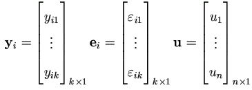
with Σ₁ = σ² I_k and Σ₂ = τ² I_n.

The reason to simulate this model is that the closed form MLE is available when all data are balanced and completely known, so we can compare simulation result easily. Since

it is easy to get the closed form MLE as below (pp.105, Searle et al, 1992).

(7.2)

The large sample variance estimates are

(7.3)

and the covariances between and ² or ² are 0.

 
7.1.2   MCEM Algorithm

First let us simplify the EM-algorithm outlined in Theorem 4.4 for this specific model. Let θ₁ = (β, σ²)' and θ₂ = τ², by equations (4.15) and (4.18) we have

(7.4)

By (4.19) the Jacobian matrices for θ₁ are

Hence the M-step (4.37) in Theorem 4.4 becomes

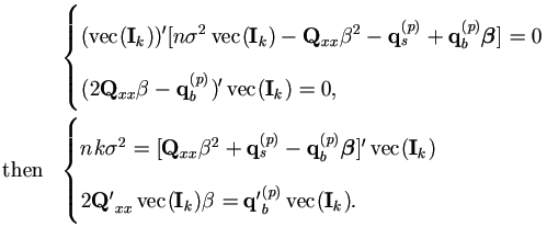
With X_i = 1_k, we have Q'_xxvec(I_k) = nk, then

Plug in q_b^(p) and q_s^(p), we have the familiar form

	(7.5)
	(7.6)

Similarly, the Jacobian matrix for θ₂ is by (4.20). From the M-step (4.38) in Theorem 4.4, we have

(7.7)

Thus the M-step in Theorem 4.4 and Theorem 4.5 can be much simplified as given below, immediately following the well simplified Gibbs sampler of Theorem 6.3.

Theorem	7.1  Given θ = (β, σ², τ²)'. For j = 1, ..., n and l = 1, ..., k, if yjl is incomplete, assume that yjl (ajl, bjl) with known ajl and bjl , possibly ± ∞.
(1).	Select staring points of u and y, and set counter i = 0. (1a). Select an arbitrary starting point u(0) = ( u1(0), ..., un(0) ). (1b). If yjl is completely known, set yjl(0) = yjl; otherwise, select an arbitrary value yjl(0) (ajl , bjl).   Let yj(0) = ( yj1(0), ..., yjk(0) )' for j = 1, ..., n.
(2).	Draw a ~ U (0, 1). Let .
(3).	For j = 1, ..., n, draw aj ~ U (0, 1) and let .
(4).	In the order of j from 1 to n draw uj(i+1) ~ U (aj(i+1), bj(i+1), where
(5).	For j = 1, ..., n, get yj(i+1) =( yj1(i+1), ..., yjk(i+1))': in the order of l from 1 to k, if yjl is known, set yjl(i+1) = yjl; otherwise draw yjl(i+1) ~ U ( ajl(i+1), bjl(i+1)), where
When i is large enough (after initial burn-in period), u(i+1) is approximately from k2(u|, θ), yj(i+1) from k1(yj|u(i+1), θ1) and (i+1) = ( y1(i+1), ..., yn(i+1), u(i+1)) from k(|, θ). Repeat steps (2-5) with i+1 to sample more points.

Theorem	7.2  The MCEM algorithm for mixed model (7.1) with incomplete data is
Step 0.	Start with values for parameters θ (0) = (β(0), σ2(0), τ2(0))' and set p = 0.
Step 1.	Select simulation sample size m and use the Gibbs sampler above to draw a sample of as (1), ..., (m) from k(|, θ(p)), where = ( y1, ..., yn, u).
Step 2.	Update θ (p+1) = (β(p+1), σ2(p+1), τ2(p+1))' as follows.
Step 3.	If converged, set = θ (p+1); otherwise return to step 1 with p + 1.

 
7.1.3   Asymptotic Dispersion Matrix of MLE

For , we have

The Jacobian Matrix Δ₁(θ₁) by (4.21) and t₁(y_i | u) by (4.16) are given as

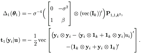
Therefore by (A.10) and (A.4),

and due to , then

Let ε_ij = y_ij - β - u_i, then by Theorem 4.3,

(7.8)

For , we have

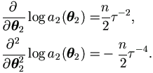
Since Δ₂(θ₂) = - τ^-4 (vec(I_n))' and t₂(u) = - ½ vec(uu'), then by Theorem 4.3,

(7.9)

Since θ = (θ₁', θ₂' )' = ( β, σ², τ²)', let ε_ij = y_ij - β - u_i, the derivatives for the combined parameter are as below.

Hence by equation (2.9), we have

Theorem 7.3   Given a sample ⁽¹⁾, ⁽²⁾, ..., ^(m) from the conditional distribution k(|,), the covariance matrix of can be approximated by

(7.10)

where S(θ) is the sample covariance matrix obtained from the m vectors

with m-1 degrees of freedom.

 
7.1.4   The Simulation

First generate a complete dataset according to the model (7.1)

y_ij = β + u_i + ε_ij           (i = 1, ..., n; j = 1, ..., k)

with the following settings:

n = 100,     k = 4 ,     β = 5,     σ = 4,     τ = 3.

That is, independently draw 100 u_i's from N (0,9) and 400 ε_ij's from N (0,16) and add them up according to the model (7.1) to get the 400 y_ij's. The summary statistics of the dataset is listed below. Due to sampling variation, the sample means of u and ε are considerably different from 0 and thus the mean of y is not equal to the theoretical value 5.

Table 7.1: Summary Statistics of Simulated Complete Data
Variable	N	Mean	Std Dev	Minimum	Maximum
u	100	0.4702	2.9635	-8.8890	6.7300
ε	400	0.1826	3.9656	-10.9641	10.8940
y	400	5.6529	4.9257	-11.4247	18.9020

 
Analysis of Complete Data

Let us compare the analysis results for the complete data by our MCEM Theorem 7.2 and by the closed form (7.2), with variance estimations based on (7.10) and (7.3), respectively. As shown in Table 7.2, the results are reasonably close to each other and our approach is comparable with the closed form solution. In fact, if increase sampling size to 10000, we can get almost identical results after about 600 iterations.

Table 7.2: Analysis Results of Complete Data
	New Approach		Closed Form
Parameter	Estimate	Std Error	Estimate	Std Error
β σ² τ²	5.6534 15.3536 8.8281	0.3573 1.2544 1.8038	5.6529 15.3465 8.8558	0.3563 1.2530 1.8221

Estimated Covariance Matrix for MLE
	New Approach			Closed Form
Parameter	β	σ²	τ²	β	σ²	τ²
β	0.1276	0.0010	-0.0025	0.1269	0	0
σ²	0.0010	1.5734	-0.3867	0	1.5701	-0.3925
τ²	-0.0025	-0.3867	3.2538	0	-0.3925	3.3201

The MCEM algorithm in Theorem 7.2 is repeated 500 times. The starting values are not very important here and we use β = -10 and σ = τ =1. The simulation sample size m ranges from 200-5000 in different EM iterations. In each EM iteration, the Gibbs sampler (Theorem 7.1) is actually run 2m times, but only the second half is counted as simulation sample while the first half is discarded as burn-in steps to ensure the convergence of the Markov Chain.

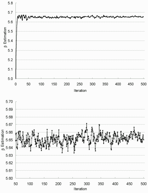
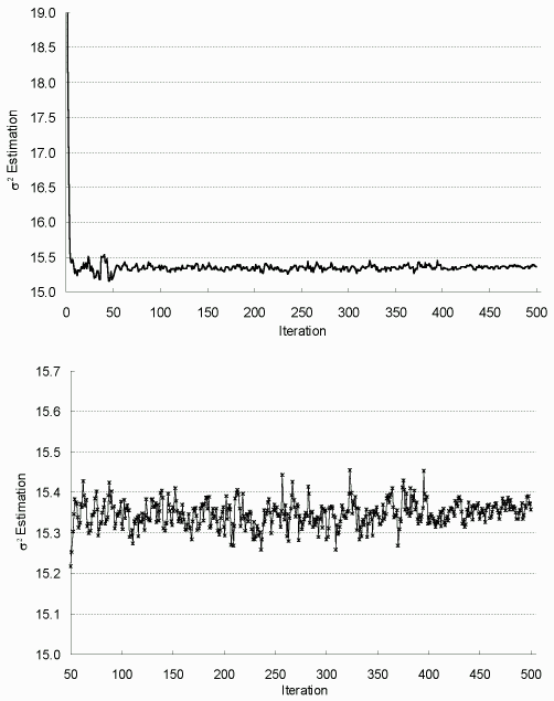
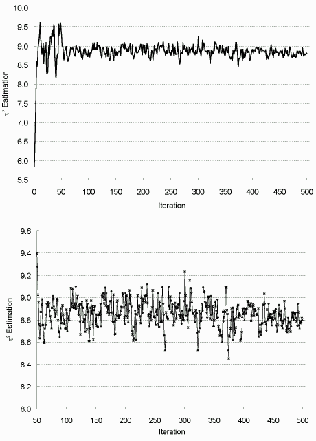
To assess the convergence of EM algorithm, parameter estimates versus iteration numbers are plotted in Figures 7.1-7.3. As shown, they stabilize quickly after about 50 iterations, then oscillate in a narrow range; and the increase of sample size m noticeably decreases the fluctuation or system variability. Based on these observations, the algorithm is terminated after 500 iterations, and the final MLE is taken as the average estimation from the last 100 iterations, with asymptotic dispersion matrix derived from the averaged Fisher information matrix.

Figure 7.1: β Estimation in Each EM Iteration (complete data)

The top figure is for all iterations and the bottom one for iterations 50-500. Sample size up from 200 to 2000 at iteration 50, and to 5000 at iteration 400.

Figure 7.2: σ² Estimation in Each EM Iteration (complete data)

The top figure is for all iterations and the bottom one for iterations 50-500. Sample size up from 200 to 2000 at iteration 50, and to 5000 at iteration 400.

Figure 7.3: τ² Estimation in Each EM Iteration (complete data)

The top figure is for all iterations and the bottom one for iterations 50-500. Sample size up from 200 to 2000 at iteration 50, and to 5000 at iteration 400.

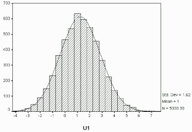
To check the convergence of the Markov Chain in the Gibbs sampler, each chain in the last EM iteration is plotted as that shown in Figure 7.4 for u₁. Apparently the chain is run to equilibrium. Figure 7.4 also shows the distribution of u₁ conditional on the observed information, which appears normal as expected.

Figure 7.4: Simulated u1 via Gibbs Sampler (complete data)

Histogram of Simulated u1 Given y

 

Analysis of Incomplete Data

We now analyze incomplete data by MCEM Theorem 7.2 and make comparison with the mid-point replaced data approach. Without loss of generality on incompleteness patterns, we assume all incomplete data are in the same interval in the simulation. Table 7.3 lists analysis results with various degrees of incomplete data by adjusting the designed incomplete interval.

It also contains the complete data results from Table 7.2 to serve as a benchmark to assess other analyses. However, strictly speaking, this benchmark can only provide very limited guidance for others, especially when incomplete data proportion is large or the incomplete ranges are rather wide. The reason is that our approach gives the MLE “averaged” over all data sets with completely known values that otherwise fall into the incomplete ranges, while the benchmark is generated from just one realization of many such possible data sets. In other words, all estimates are MLEs, but from different data sets. They do not have to be the same, as they often should not.

Table 7.3: Analysis of Incomplete Data
Incompleteness			New Approach		Mid-Point Replaced
Interval	%	Parameter	Estimate	Std Error	Estimate	Std Error
	0%	β σ² τ²	5.6534 15.3536 8.8281	0.3573 1.2544 1.8038	5.6529 15.3465 8.8558	0.3563 1.2530 1.8221
(-1, 1)	11%	β σ² τ²	5.6285 15.5621 8.8982	0.3592 1.2751 1.8222	5.6190 15.6142 8.9319	0.3583 1.2749 1.8430
(-3, 3)	27%	β σ² τ²	5.6585 14.9900 9.2364	0.3645 1.2860 1.8784	5.4862 15.9036 9.4405	0.3663 1.2985 1.9249
(-5, 5)	42%	β σ² τ²	5.6651 15.3044 9.0407	0.3715 1.4625 1.9420	5.0088 18.3367 9.4994	0.3753 1.4972 2.0266
(-6, 6)	51%	β σ² τ²	5.5375 16.1990 9.3129	0.3890 1.6758 2.1093	4.5267 20.1392 9.4888	0.3811 1.6444 2.0947
(-8, 8)	67%	β σ² τ²	5.5723 14.5307 10.2261	0.4420 1.9121 2.5264	3.5443 20.0763 9.4264	0.3801 1.6392 2.0836
(-10, 10)	82%	β σ² τ²	5.3577 13.8621 11.5601	0.5843 2.6334 3.3122	2.2740 18.0623 6.8578	0.3372 1.4748 1.6502
(-12, 12)	91%	β σ² τ²	6.5369 9.7932 7.9524	1.0154 3.1534 3.7757	1.3390 13.5592 3.7677	0.2675 1.1071 1.0494

Monte Carlo Simulation Settings
Simulation	No. of EM Iterations	Sample Size m (per EM Iteration)	Burn-in
0-42%	500	200 (1-49), 2000 (50-399), 5000 (400-500)	m
51-67%	800	500 (1-599), 5000 (600-800)	m
82%	1000	500 (1-799), 5000 (800-1000)	m
91%	4000	500 (1-1999), 5000 (2000-4000)	min(m,1000)

As expected, our approach consistently outperforms the mid-point replacement method, especially when the incomplete proportion is large. Also, the estimation for β from the mid-point replaced data is always smaller than that from MCEM approach. This is due to that the complete data mean is 5.6529 (see Table 7.1), so the mid-point 0 should be less than the expectation over the incomplete interval.

What is truly remarkable is that even under situations of extremely heavy incompleteness (50-80%), we can still obtain rather good estimations. At the essence of our approach, for those incomplete data we still fully take in all information contained therein by integrations. Therefore theoretically, with proper distribution and other model assumptions, a reasonable MLE can be expected even under extreme cases. On the other hand, the incomplete data proportion cannot be too high in order to have any meaningful analysis. This is reflected by the fact that when the incomplete proportion increases, the standard errors of estimations will become larger as well, or the EM iterations will take forever to stabilize.

Parallel to Figures 7.1-7.3, as two examples, we plot Figures 7.5 and 7.6 to assess the convergence of the EM algorithm when incomplete proportion is 42% and 82% respectively. As shown on these figures, (1) the MCEM scheme stabilizes quickly, then oscillates in a narrow range; (2) the increase of sampling size m noticeably decreases the system variability; and (3) the heavier in the incompleteness, the more EM iterations and larger sample sizes we need.

Figure 7.5: Estimations in Each EM Iteration (42% incomplete)

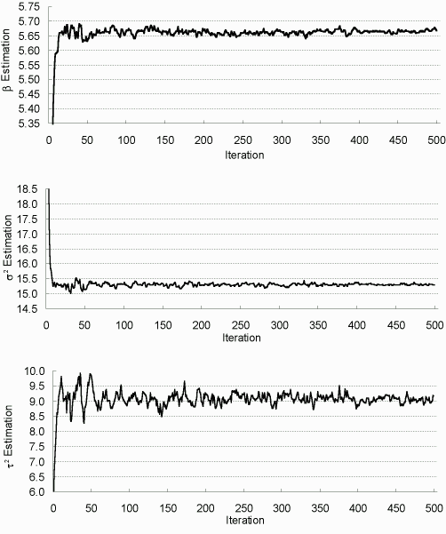Sample size up from 200 to 2000 at iteration 50, to 5000 at iteration 400.

Figure 7.6: Estimations in Each EM Iteration (82% incomplete)

Sample size is increased from 500 to 5000 at iteration 800.

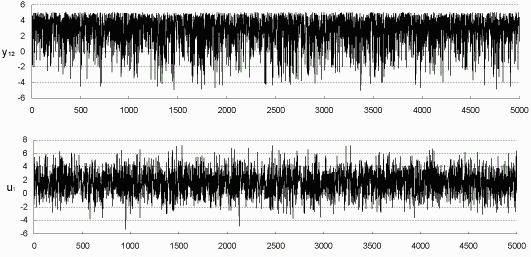
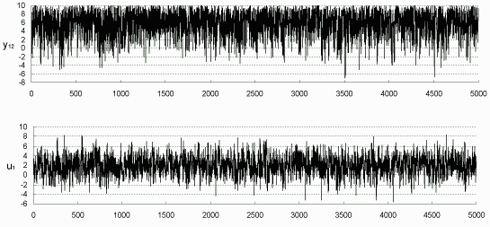
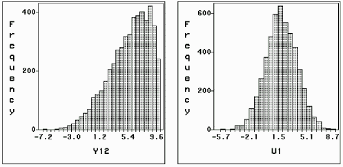
Also as in Figure 7.4, the Markov Chains from the last EM iteration can be plotted to check the convergence of sampling distribution. For example, in the simulation with 42% incomplete data, y₁₂ is only known within (-5, 5), so we plot the chain in Figure 7.7 for y₁₂, as well as for u₁. Apparently the two chains are run to equilibrium. Figure 7.7 also shows the distributions of y₁₂ and u₁ conditional on the observed information. Parallel Figure 7.8 is for the simulation with 82% incomplete data.

Figure 7.7: Simulated y12 (-5, 5) and u1 (42% incomplete)

Histograms of Simulated y12 and u1

Figure 7.8: Simulated y12 (-10, 10) and u1 (82% incomplete)

Histograms of Simulated y12 and u1

This is a very computation intensive approach as expected. Except the extreme case of 91% incomplete, each simulation takes about 0.5-3 hours running SAS 7.0 system in a Pentium 450 MHz PC (The case of 91% takes about 16 hours). As mentioned earlier, our simulation settings are quite conservative. Lowering the burn-in rate of 100% to around 1000 could halve the running time. In fact, the Gibbs sampler in Theorem 7.1 is very efficient, considering that the total number of sampled values could be as high as 10⁹ when the proportion of incomplete data is extremely high. To get more accurate estimations, the simulation sample size during late stages seems to be the most important factor.

 
7.2   The Motivation Data with Random Intercept

As an example with practical data, let us analyze the motivation data introduced in section 1.1. There are 40 subjects with 6 measures per subject in the data. As shown in Table 1.1, these 240 measures are almost evenly distributed in the three categories: complete, censored and totally missing.

7.2.1   The Model

Let us fit the following simple mixed model with some y_ij missing or incomplete,

yij = β0 + β1 xj + ui + εij

(i = 1, ..., n; j = 1, ..., k)

(7.11)

where n=40, k=6, y_ij= ln((PAHDNA)_ij+1) for subject i at time j, and x_j is number of weeks after quit smoking at time j. Assume u_i ~ N (0, τ²), ε_ij ~ N (0, σ²), and all u_i's and ε_ij's are independent of each other. The two fixed effects are β₀ and β₁ , and u_i's are n random effects. Rewrite it in the matrix form as in equation (4.2),

y_i = Xβ + Z_iu + e_i,      (i = 1, ..., n)

where Z_i = [ 0_k×(i-1)   1_k   0_k×(n-i) ]_k×n and

with Σ₁ = σ² I_k and Σ₂ = τ² I_n.

 
7.2.2   MCEM Algorithm

First let us simplify the EM-algorithm outlined in Theorem 4.4 for this specific model. Let θ₁ = (β₀, β₁, σ²)' and θ₂ = τ², by equations (4.15) and (4.18) we have

(7.12)

By (4.19) the Jacobian matrices for θ₁ are

Hence the M-step (4.37) in Theorem 4.4 becomes

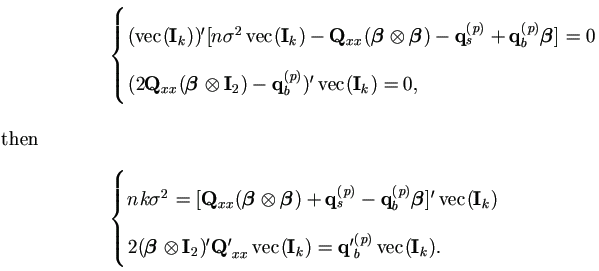
By (A.4), (β I₂)' Q'_xxvec(I_k) = n X'X β and (β β )' Q'_xxvec(I_k) = n β ' X'X β, then

(7.13)

Plug in q_b^(p) and q'_s^(p), we have the familiar form

	(7.14)
	(7.15)

Similarly the Jacobian matrix for θ₂ is by (4.20). Then from the M-step (4.38) in Theorem 4.4, we have

(7.16)

Hence the M-step in Theorem 4.4 and Theorem 4.5 can be much simplified as given below, immediately following well simplified Gibbs sampler in the E-step of Theorem 6.3.

Theorem	7.4  Provided that θ = (β0, β1, σ², τ²)' is known. For j = 1, ..., n and l = 1, ..., k, if yjl is incomplete, assume that yjl (ajl, bjl) with known ajl and bjl , possibly ± ∞.
(1).	Select staring points for u and y, and set counter i = 0. (1a).   Select an arbitrary starting point u(0) = ( u1(0), ..., un(0) ). (1b).   If yjl is completely known, set yjl(0) = yjl; otherwise, select an arbitrary starting value yjl(0)(ajl , bjl).   Let yj(0) = ( yj1(0), ..., yjk(0) )' for j = 1, ..., n.
(2).	Draw a ~ U (0, 1). Let .
(3).	For j = 1, ..., n, draw aj ~ U (0, 1), let .
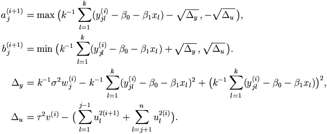
(4).	In the order of j from 1 to n draw uj(i+1) ~ U (aj(i+1), bj(i+1), where
(5).	For j = 1, ..., n, get yj(i+1) =( yj1(i+1), ..., yjk(i+1))' as follows. In the order of l from 1 to k, if yjl is known, set yjl(i+1) = yjl; otherwise draw yjl(i+1) ~ U ( ajl(i+1), bjl(i+1)) and denote μjl=β0+β1xl+uj , where
When i is large enough (after initial burn-in period), u(i+1) is approximately from k2(u|, θ), yj(i+1) from k1(yj|u(i+1), θ1) and (i+1) = ( y1(i+1), ..., yn(i+1), u(i+1)) from k(|, θ). Repeat steps (2-5) with i+1 to sample more points.

Theorem	7.5  The MCEM algorithm for the mixed model (7.11) with incomplete data is given below.
Step 0.	Start with values for parameters θ (0) = (β '(0), σ2(0), τ2(0))' and set p = 0.
Step 1.	Select simulation sample size m and use the Gibbs sampler above to draw a sample of as (1), ..., (m) from k(|, θ (p)), where = ( y1, ..., yn, u).
Step 2.	Update θ (p+1) = (β '(p+1), σ2(p+1), τ2(p+1))' as follows.
Step 3.	If converged, set = θ (p+1); otherwise return to step 1 with p + 1.

Note that for matrix X'X and its inverse if not all x_j's are equal, we have

For any vector a = (a₁ a₂)', we have a'X'Xa =(a₁+ a₂ x_j )², in particular,

 
7.2.3   Asymptotic Dispersion Matrix of MLE

Since , then

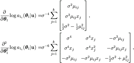
where μ_ij = β₀ + β₁ x_j + u_i.

The Jacobian Matrix Δ₁(θ₁) by (4.21) and t₁(y_i|u) by (4.16) are

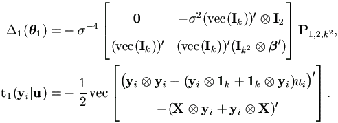
Therefore by (A.10) and (A.4),

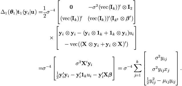
Due to , then

Let ε_ij = y_ij - (β₀ + β₁ x_j + u_i ), then by Theorem 4.3,

(7.17)

For , we have

Note that Δ₂(θ₂) = - τ^-4 (vec(I_n))' and t₂(u) = - ½ vec(uu'), then by Theorem 4.3,

(7.18)

Then the derivatives for parameters θ = (θ₁', θ₂' )' = ( β₀, β₁, σ², τ²)' are

where ε_ij = y_ij - (β₀ + β₁ x_j + u_i ), and

Hence by equation (2.9), we can use the same result as in Theorem 7.3. Given a sample ⁽¹⁾, ⁽²⁾, ..., ^(m) from the conditional distribution k(|, ), the covariance matrix of can be approximated by

(7.19)

where S(θ) is the sample covariance matrix obtained from the m vectors

with m-1 degrees of freedom.

 
7.2.4   Analysis via Mid-point Replacement

For comparison purpose, the mid-point replaced data is also analyzed. As shown in Table 1.1, there are 81 missing values out of total 240 measures. Thus the analysis uses the remaining 159 measures, and 75 out of these 159 are censored and replaced.

The dependent variable is PAH-DNA adduct level plus 1 then with natural log transformation, i.e. y = ln(PAHDNA+1). The legitimate range for PAHDNA is any positive value, however, if that value is 2 or below, it would be undetectable in laboratory analysis and yield an incomplete observation censored in the interval (0, 2]. Since in the mid-point replaced data such observations will be replaced by 1, then PAHDNA is always 1 or greater unless it is missing, and there is no need to add 1 before log-transformation. However, adding 1 would not change much on the results of this analysis, but it will enhance the performance of our MCEM scheme. After adding 1, the transformed incomplete range would be (0, ln3] instead of (-∞, ln2] otherwise. It seems easier to sample from a narrow interval.

The only fixed effect besides the intercept is x_j, the number of weeks after quit smoking at time j. This is a subject-independent measure and has 6 levels as 0, 10, 36, 62, 88, 114. Since the effect of this covariate is rather small in absolute value, we rescale this covariate by a factor of 1/100 in order to make results more stable and comparison easier with more significant digits. Consequently, keep in mind that x_j = 0, 0.10, 0.36, 0.62, 0.88, 1.14 in subsequent analyses.

After replacing censored values and excluding missing measures, the resulting dataset is unbalanced. Its MLEs can be obtained via Proc MIXED in the SAS system 7.0, which uses Newton-Raphson algorithm. The results together with SAS syntax are shown in Table 7.4.

Table7.4: Analysis of Data with Replacement: Random Intercept Model
Parameter   Estimate   Std Error β0 1.7002 0.1028 β1 -0.4822 0.1770 σ² 0.5874 0.0775 τ² 0.1123 0.0666	SAS Syntax proc mixed method=ml covtest; class id; model y=week /s; random intercept / subject=id; run;

 
7.2.5   Analysis via MCEM Algorithm

Now let us analyze the data using the MCEM algorithm outlined in Theorem 7.5 with the Gibbs sampler of Theorem 7.4. The asymptotic standard error and covariance of MLE will be estimated by (7.19).

There are two types of incomplete measures in this dataset, 75 censored measures as y_ij (0, ln3] and 81 missing measures as y_ij (0, +∞). Note that even for the missing measures, the range is not (-∞, +∞) as we know ln(PAHDNA+1) > 0. This “extra” information will be utilized in our analysis as well for what it is worth. We do not throw away any observations, even those with partial information as little as contained in these 81 missing measures.

To get the MLEs for the original 240 measures without any modification, we run the MCEM algorithm 800 times with arbitrary starting values as β₀ = β₁ = 0 and σ² = τ² = 1. The sample size m for each EM iteration is set to 500 for iterations 1-399, 1000 for iterations 400-599 and 5000 for iterations 600-800. Also the burn-in length is always set to 500. The reason that these simulation parameters are set so high is due to the fact that the original dataset have rather small sample size but with heavy missing (about 1/3) and censoring (about another 1/3). Higher settings will stabilize the process quicker and narrow the swinging range. The analysis result is listed in Table 7.5.

Table 7.5: Analysis via MCEM Algorithm
Parameter	Estimate	Std Error
β0	1.6765	0.1015
β1	-0.3131	0.1661
σ²	0.5992	0.0811
τ²	0.0875	0.0585

As in the simulations, in order to filter out random fluctuations, the final MLE is taken as the average estimation from the last 100 EM iterations, and the asymptotic dispersion matrix is derived from the averaged Fisher information matrix. As known from prior simulations and also shown in the diagnostic Figure 7.10, the increase in simulation sample size m could effectively decrease this fluctuation but with increased computing cost.

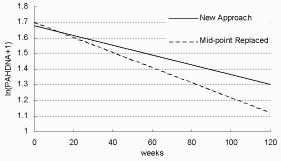
It is expected that the results in Table 7.4 have bias introduced by data replacement, but after comparison with Table 7.5 , that bias seem not noticeable in estimating β₀ and σ², thus it appears that the simple mid-point replacement is not a bad practice in estimating the intercept (β₀) for current data. On the other hand, there are rather obvious disparities in the estimations of β₁ and τ², particularly for the slope β₁. It is not unexpected as so many measures are censored or missing in the original data. The estimation of β₁ in Table 7.5 shows a slower decline, which implies that the

Figure 7.9: PAH-DNA Decline over Time

conditional expectations for censored or missing observations are likely larger than the mid-point value 1 used in the PAH-DNA measure replacement, especially in late time points. The reasons for this could be very complicated, but the following three observations could be helpful to explain: (1) the censoring interval of PAH-DNA measure is (0, 2), while its mean is about 8.3, so a value larger than 1 seems more reasonable and is likely generated in simulation. This observation is suggestive but not conclusive since conditional distributions in stead of marginal distributions were used in simulations; (2) from Table 1.1 during late time points the proportion of censored or missing data is much larger, so those measures were affected more severely than early measures, which causes a flatter slope in MCEM algorithm; (3) for missing observations, we used the expectations over (0, +∞) instead of (-∞, +∞), which makes the data more accurate but tends to produce slightly larger expectations. Again this especially affects late times points where missing is heavier.

To assess the convergence of the MCEM algorithm, as Figures 7.1-7.3 and 7.5-7.6 , parameter estimates versus iteration numbers are plotted in Figure 7.10. As shown, they stabilize quickly after about 50 iterations, then oscillate in a narrow range; and the increase of sample size m noticeably decreases the fluctuation or system variability.

Figure 7.10: Parameter Estimations in Each EM Iteration

iterations

Sample size up from 500 to 1000 at iteration 400, and to 5000 at iteration 600.

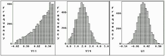
To check the convergence of Markov Chains in the Gibbs sampler, the chains of simulated variables in the last EM iteration could be plotted as in Figure 7.4 and 7.7-7.8. As an example, we plot the following three chains in Figure 7.11 for the first subject: y₁₁ is censored in (0, ln3); y₁₄ is missing though we know y₁₄ > 0 and u₁ is a unobservable random effect. Apparently all of these chains are run to equilibrium. Figure 7.11 also shows the conditional distributions given all observed information.

Figure 7.11: Simulated y11 (0, ln3), y14 (0, +∞) and u1 (-∞ +∞)

Histograms of Simulated y11, y14 and u1

This MCEM analysis takes about 1.5 hours running SAS 7.0 system in a Pentium 450 MHz PC. As mentioned earlier, our simulation settings are quite conservative. As shown by these figures above, the algorithm starts to stabilize within just about 50 iterations, which could take only a few minutes. However, within certain limit, the higher the settings are, more accurate the results will be.

 
7.3   The Motivation Data with Random Slope

Since the variation among slopes has more important meaning biologically, now we analyze the motivation data again with random slope. Due to small sample size of the data, the intercept is kept fixed in this model. Otherwise the estimations cannot be stable, since the model would have 80 random effects, but the dataset has only 84 complete measures.

7.3.1   The Model

Let us fit the following mixed model with random slope as

yij = β0 + β1 xj + ui xj + εij

(i = 1, ..., n; j = 1, ..., k)

(7.20)

where n=40, k=6, y_ij= ln((PAHDNA)_ij+1) for subject i at time j, and x_j is number of weeks after quit smoking at time j. The two fixed effects are β₀ and β₁ , and u_i are n random effects. Assume u_i ~ N (0, τ₁²), ε_ij ~ N (0, σ²), and all u_i's and ε_ij's are independent of each other. Rewrite it in the matrix form as in equation (4.2),

y_i = Xβ + Z_iu + e_i,      (i = 1, ..., n)

where

Zi = [ 0k×(i-1)   [x1 ... xk]'   0k×(n-i) ]k×n

with Σ₁ = σ² I_k and Σ₂ = τ₁² I_n.

 
7.3.2   MCEM Algorithm

Let θ₁ = (β₀, β₁, σ²)' and θ₂ = τ₁². Denote _ij = y_ij - u_i x_j. Parallel to the random intercept only model, it is easy to have

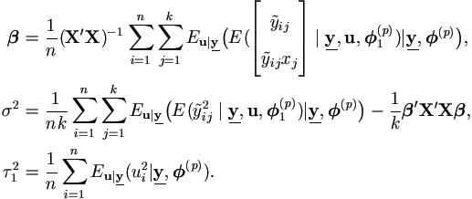
Hence we have the following much simplified Gibbs sampler and EM-Algorithm.

Theorem	7.6  Provided that θ = (β0, β1, σ², τ1²)' is known. For j = 1, ..., n and l = 1, ..., k, if yjl is incomplete, assume that yjl (ajl, bjl) with known ajl and bjl , possibly ± ∞.
(1).	Select staring points for u and y, and set counter i = 0. (1a).   Select an arbitrary starting point u(0) = ( u1(0), ..., un(0) ). (1b).   If yjl is completely known, set yjl(0) = yjl; otherwise, select an arbitrary starting value yjl(0)(ajl , bjl).   Let yj(0) = ( yj1(0), ..., yjk(0) )' for j = 1, ..., n.
(2).	Draw a ~ U (0, 1). Let
(3).	For j = 1, ..., n, draw aj ~ U (0, 1), let .
(4).	Denote jl(i) = yjl(i) - β0 - β1xl for j = 1, 2, ..., n; l = 1, 2, ..., k. In the order of j from 1 to n draw uj(i+1) ~ U (aj(i+1), bj(i+1), where
(5).	For j = 1, ..., n, get yj(i+1) =( yj1(i+1), ..., yjk(i+1))' as follows. In the order of l from 1 to k, if yjl is known, set yjl(i+1) = yjl; otherwise draw yjl(i+1) ~ U ( ajl(i+1), bjl(i+1)) and denote μjl=β0+β1xl+ujxl , where
When i is large enough (after initial burn-in period), u(i+1) is approximately from k2(u|, θ), yj(i+1) from k1(yj|u(i+1), θ1) and (i+1) = ( y1(i+1), ..., yn(i+1), u(i+1)) from k(|, θ). Repeat steps (2-5) with i+1 to sample more points.

Theorem	7.7  The MCEM algorithm for the mixed model (7.20) with incomplete data is given below.
Step 0.	Start with values for parameters θ (0) = (β '(0), σ2(0), τ12(0))' and set p = 0.
Step 1.	Select simulation sample size m and use the Gibbs sampler above to draw a sample of as (1), ..., (m) from k(|, θ (p)), where = ( y1, ..., yn, u).
Step 2.	Let ij(l) = yij(l) - ui(l) xj for l = 1, 2, ..., m. Update θ (p+1) = (β '(p+1), σ2(p+1), τ12(p+1))' as follows.
Step 3.	If converged, set = θ (p+1); otherwise return to step 1 with p + 1.

 
7.3.3   Asymptotic Dispersion Matrix of MLE

It is easy to get following results parallel to those for the random intercept only model.
For θ₁, let ε_ij = y_ij - (β₀ + β₁ x_j + u_i x_j), then

For θ₂, it is easy to have

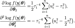
Then the derivatives for parameters θ = (θ₁', θ₂' )' = ( β₀, β₁, σ², τ₁²)' are given by

Hence we can use the same result as in Theorem 7.3 to approximate var().

 
7.3.4   Data Analysis Results

To analyze the data using Theorem 7.5, we run the MCEM algorithm with the same settings as in the random intercept only model. Similarly, for comparison purpose, the mid-point replaced data is also analyzed via SAS Proc MIXED. Both results are shown in Table 7.6.

Table7.6: Data Analysis Results with Random Slope Model
via MCEM Algorithm Parameter Estimate Std Error β0 1.6686 0.0952 β1 -0.2792 0.1746 σ² 0.6825 0.0792 τ1² 0.0207 0.0504	via Mid-point Replacement Parameter Estimate Std Error β0 1.6928 0.0932 β1 -0.4549 0.1992 σ² 0.6597 0.0809 τ1² 0.1342 0.1636

By comparing the results via these two approaches, we have similar findings just as those from the random intercept only model. For current data, the estimations of β₀ and σ² are fairly close, but the estimations of β₁ and τ₁² are quite different. Also, both approaches show that the estimation of τ₁² is not significant, which suggests that the slope might not be random in current data. However, we need interpret the Std Error estimation with caution since it is based on large sample size assumption but current sample size is not very large.

To assess the convergence of the MCEM algorithm, parameter estimates versus iteration numbers can be plotted in as in Figure 7.10. To check the convergence of Markov Chains in the Gibbs sampler, the chains of simulated variables in the last EM iteration could be plotted as in Figure 7.11. All of these plots are similar to those for the random intercept only model and supportive for the claim of convergence.

This MCEM analysis takes about 2 hours running SAS 7.0 system in a Pentium 450 MHz PC. As computing power advances rapidly nowadays, this and other computation intensive methods should become more and more affordable.
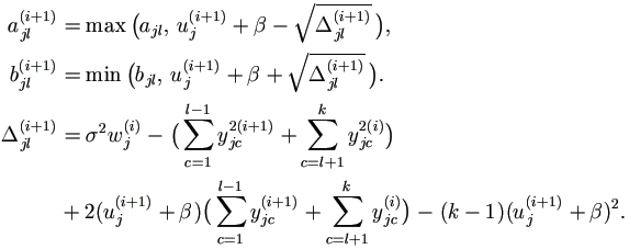
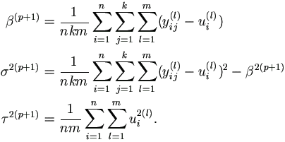