Copyright (c) B.Achutha 1992 - 2000 Malaysia

Frequency Distribution

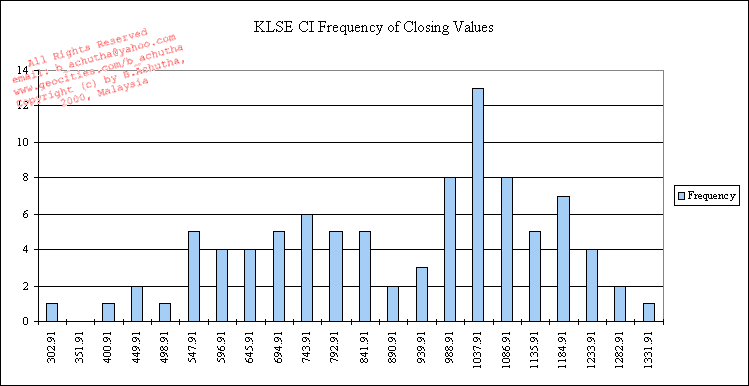
The state boundaries are mathematically derived from statistical techniques. From my experience, this is the only statistical analysis that I reccommend for market movements. In the graph below we can observe that there are three states. The first is less then 496, the second lies between 496 and 890 and the third is above 890. This distribution is for the closing values of the KLSE Composite Index. The boundaries of the individula states are derived from the +/- 1.5 or 2 sigma (std dev).