Chapter 5   Special Models For Normal Data

In this Chapter, we deal with some important special cases of mixed models with Normal distribution. This will serve as illustrative examples of applying the EM-Algorithm (Theorem 4.4) from prior chapter. For certain models, it will also provide us some comparisons with existing results in the literature.

 
5.1   Univariate Models with Censored Data

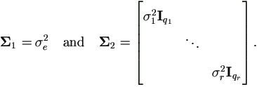
For better understanding, we first demonstrate the algorithm when outcome is a scalar, i.e. k =1. Models for errors-in-variable have this form when there is no censoring. Scalar y_i's are assumed independent given u, just as assumed before for vector y_i. Specifically, let Σ₁ = σ_e², and in most circumstances the parameters of interest for y_i|u can be assumed as

  by equation (4.15).

Even under this simplified setting, we can still model essentially all models that can be handled by the general setting above by adjusting Σ₂, covariance structure of u.

By (4.19), the Jacobian matrices for θ₁ is

Now that is a non-singular matrix, we may drop this term from M-step (4.37), which becomes

This can be further simplified as the solution of the following equation system.

From the second equation above, we know that q_b^(p) = 2Q_xx(β I_p), plug this into the first equation, we get

	(5.1)
	(5.2)

Since each X_i is a matrix of order k × p, we may stack all X_i's for i =1, 2, ..., n to form a sample-wise design matrix of order nk × p as

When k = 1, we have the following relationship

This is evident when treat as a (block) vector with each entry being one of the (row) vectors X_i. Then by (A.4),

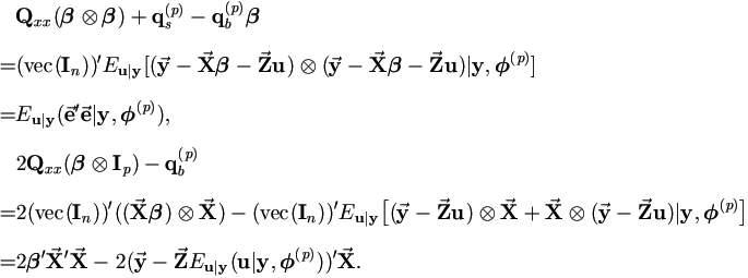
The last equality is due to that 'β is a column vector. Hence (5.1) leads to 'β =½ q'_b^(p). That is,

(5.3)

Since then by (5.2),

(5.4)

Therefore the M-step (4.37) can be replaced by these much simpler equations (5.3) and (5.4).

 
5.2   Mixed Models without Censored Data

We now present the algorithm for the mixed model for complete data with multivariate normal distribution. The algorithm is different from that is given by Dempster, Rubin and Tsutakawa (1981).

If all components of every y_i are completely observed, there is no need to calculate conditional expectations for y_i, so we can simplify the E-step substantially. Note that now the observed data = y. Therefore we have

Theorem 5.1.   The EM-algorithm for mixed model with complete data from normal distribution can be defined as

Step 0.	Start with values for parameters 1(0) and 2(0). Set p = 0.
Step 1.	(E-step) Calculate as given in (4.26) and (4.24), (5.5)
Step 2.	(M-step) Determine (p+1) by 1(p+1) = 1(θ1(p+1)) as the solution of . (5.6) and 2(p+1) = 2(θ2(p+1)) as the solution of Δ2(θ2)vec(Σ2) = Δ2(θ2) su(p). (5.7)
Step 3.	If converged, set = (p+1); otherwise increase p by 1 and return to step 1.

 
Special Case: A Univariate Mixed Model without Censored Data

Now we show that the algorithm above agrees with the EM-algorithm of section §2.2, where all y_i are scalars (i.e. k = 1). Follow the same distributional assumptions and use notations in that section, we have

Then the parameters of interest are

Also by equations (4.15) and (4.18), we have

In order to be comparable to section §2.2, we stack all individual matrices as below to form the sample-wise matrices corresponding to y, X, Z, e of that section.

Then the model (4.1) can be written as

For Jacobian matrices, by (4.19),

Note that now is a non-singular matrix, so we may drop this term from M-step (5.6), which becomes

(5.8)

It is easy to verify that Q_xx = (vec(I_n))'( ) due to k =1. And by (5.5) we have

Then by above relationships and (A.4),

	(5.9)
	(5.10)

Therefore by (5.8) and (5.9), n vec(Σ₁) = . Since Σ₁ = σ_e², we have

σ_e² = /n.

By (5.8) and (5.10), . Hence

These results agree with those in the EM-algorithm of section §2.2.

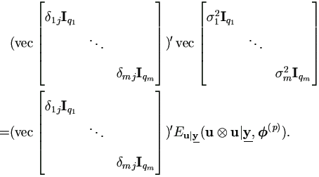
Let δ_ij be the Kronecker symbol, then

(5.11)

where for j =1, 2, ..., r,

Now apply to equation (5.7), we get

Then for each j =1, 2, ..., r,

By (A.2) and (A.4),

That is, q_jσ_j² = E_u|y u'_ju_j|y, ^(p)). Therefore for j =1, 2, ..., r,

σ_j² = E_u|y u'_ju_j|y, ^(p))/q_j.

These results again agree with those in the EM-algorithm of section §2.2.

 
5.3   Pure Random Effect Models

Pure random effect model is a special case of mixed models in equation (4.1), but without fixed effects. First, we derive the EM-algorithm based on Theorem 4.4 for this special case, and then compare the results with that from Pettitt's approach (Pettitt, 1986) as outlined in section §1.4.2.

Since X = 0, the model becomes y = Zu + e. Theorem 4.4 becomes much simpler as many terms go to 0. Since q_b^(p) = Q_xx = 0, we have

Lemma 5.1.   The M-step for pure random effects model from normal distribution is as follows. Determine ^(p+1) by ₁^(p+1) = ₁(θ₁^(p+1)) as the solution of

Δ_{σ ^-}(θ₁)(n vec(Σ₁) - q_s^(p) ) = 0,

and ₂^(p+1) = ₂(θ₂^(p+1)) as the solution of

Δ₂(θ₂) (vec(Σ₂) - s_u^(p) ) = 0.

Lemma 5.2.

Proof.   Note that e_i = y_i - Z_iu and by (4.26),

Then the desired result will be obtained by applying (A.6).

Lemma 5.3.

s_u^(p) = vec ((uu'|, ^(p))).

Proof.   By definition (4.24), s_u^(p) = (uu|, ^(p)). By (A.6), uu = vec(uu'), hence the lemma holds.

Theorem 5.2.   EM-algorithm for pure random effects model from normal distribution is defined below. Note that Σ₁ = Σ₁(θ₁) and Σ₂ = Σ₂(θ₂).

Step 0.	Start with values for parameters 1(0) and 2(0). Set p = 0.
Step 1.	(E-step) Calculate (eie'i|, (p)) and (uu'|, (p)) as given above.
Step 2.	(M-step) Determine (p+1) by 1(p+1) = 1(θ1(p+1)) as the solution of (5.12) and 2(p+1) = 2(θ2(p+1)) as the solution of Δ2(θ2) vec(Σ2 - (uu'|, (p))) = 0. (5.13)
Step 3.	If converged, set = (p+1); otherwise increase p by 1 and return to step 1.

 
5.3.2   Special Case: Pettitt's Model

Now compare the results based on Theorem 5.2 and that from section 2 of Pettitt's paper (1986) as outlined in section §1.4.2 for the usual random effects models.

Since Σ₁=σ²I_k, let θ₁=σ², then Σ₁(θ₁)=θ₁I_k. From equation (4.15), we have ₁(θ₁) = vec() = θ₁^-1 vec(I_k). Therefore the Jacobian matrix in (4.19) is

Now equation (5.12) becomes

By equation (A.2), it becomes

Since tr(e_ie'_i) = e'_ie_i, then n tr(Σ₁) = . Since tr(Σ₁) = kσ², and let e=(e₁', ..., e_n')', we have

nkσ² = .

This agrees with Pettitt's result as nk here is equal to q_k+1 in Pettitt's paper.

In order to compare results for other random components, let us map Pettitt's model into our framework. To avoid ambiguity over notations, here we use m to denote k in that paper. Now we have

and by equation (4.18) we have ₂(θ₂)=vec(), where

Let δ_ij be the Kronecker symbol, then for Δ₂,

(5.14)

where for j =1, 2, ..., m,

Apply to equation (5.13), we get

Then for each j =1, 2, ..., m,

By (A.2) and (A.4) in the Appendix,

Therefore, for i =1, 2, ..., m,

q_iσ_i² = (x'_ix_i|, ^(p)).

These results again agree with those from Pettitt's paper.

All results agree on that the E-step must be carried out for the expectation of x'_ix_i or e'e with respect to the conditional distribution of x or e given . The core calculation involved is in fact about the conditional expectations for y_i and y_i y_i over incomplete observations as given in equations (4.30) and ((4.31). They are equivalent to the formulae given in section 2.2 in Pettitt's paper. However, the calculation is very complicated in general. The method provided by Pettitt in section 3 circumvents this difficulty for a simple type of model. In fact it is only easily available when the structure of variance-covariance matrix is simple. In general, we must use numerical methods to approximate multi-dimensional integrals.