Excel 2000 Module 3
Formulas & Functions
With
Excel, it's easy to perform common calculations. In addition
to adding, subtracting, multiplying, and dividing, you can calculate
the total and compute the average of a set of values.
Click <File>
<Open>
Practice M2Ex
Click <Sheet1>
Rename <Sheet1>
to <M2Ex>
Click
Cell
A7
Type
Total
Formula Concepts
A formula is the written expression of a calculation to be performed by Excel. When you enter a formula into a cell, the formula is stored internally while the calculated result appears in the cell.
Excel Mathematical Operators
(.......) any computation in the bracket;
^ exponential such as 3^2 is 3²;
* multiplication such as 3*2;
/ division such as 3/2;
+ addition such as 3+2;
- subtraction such as 3-2.
Operators and Priority Rules
Calculation in Excel follows the Priority Rules in the Operators
( ); ^ ; * or / ; + or -
Priority 1 : ( )
Priority 2 : ^
Priority 3 : * or / first-come-first-serve
Priority 4 : + or - first-come-first-serve
e.g. =1+2*3+(2*3/3)
Step 1 (Priority 1): 2*3 first then divided by 3
Step 2 : 2*3 + Step 1 sub total
Step 3 : 1 + Step 2 sub total
Creating Formulas
Creating a formula is similar to entering text and numbers in cells. To begin, you select the cell in which you want the formula to appear. You can use one of two methods to create the formula.
In
the first
method,
you type the formula, including cell addresses, constant values,
and mathematical operators, directly into the cell. To mark the
entry as a formula, you start by typing an equal = sign.
Click Cell
B8
Type at the Formula bar B5+B6
In
the second
method,
you start by clicking an equal
= sign (<Edit>
button at the Formula bar), then paste the references for
a cell or range of cells in the Formula bar. You then complete
the formula by typing any operators, constant values, or parentheses.
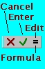
When Excel is in Edit mode, three buttons appear to the left of
the Formula bar :
<Cancel>, <Enter>, and <Edit>.
Click
Cell
C8
Click Cell C5
Type +
Click Cell C6
Click <Enter>
on the Formula bar
Copying Formulas
When you change your mind about the placement of the Formula of a cell, you can change the way you've placed data in your worksheet.
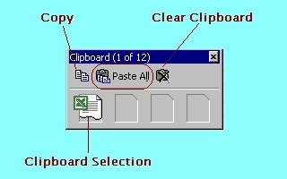
Copy & Paste, Cut & Paste

Alternatively Use Clipboard
Menu, Point and click <View><Toolbars> :
click Clipboard
Alternatively Use Fill Handle
When you select a cell with a formula and drag the Fill handle, Excel changes the cell references in the formula to match those of the column or row to which it has been copied.

Select Cell C8, drag Fill handle to D8
Editing Formulas
Editing a formula that you have already created is easy and similar to editing the contents of any other cell.
Double-click the cell, type your changes directly in the cell, and <Enter>
When Excel is in Edit mode, three buttons appear to the left of the Formula bar :
<Cancel>, <Enter>, and <Edit>.

Click the cell, click in the Formula bar, type your changes, click <Enter or => button on the Formula bar.
Click the cell, click <Edit or => Formula button, type your changes in the Formula bar, click <Enter> button on the Formula bar.
Using Absolute and Relative Cell References
An absolute reference refers to the address of a specific cell. A relative reference refers to a cell that is a specific rows and columns from the cell that contains the reference.
Click <Sheet2>
Rename <Sheet2> to <Mixed Addressing>
Practice M3Ex
Click Cell C4
Create the Formula
You will notice how the relative cell referencing error will happen when you copy or use Fill handles on the formulas.
Do you notice how the absolute cell referencing for column B does when you copy formulas across.
Use <F2> key to examine the formula
Press <Esc> to quit
To correct the error, we edit the formula.
Example : B1 (Column B Row 1)
$B$1 absolute reference
Use <F2> key to examine the formula
Press <Esc> to quit
No error if we copy formula across or downwards
Example : B4 (Column B Row 4)
$B4 absolute reference to Column B, but relative reference to Row 4
Use <F2> key to examine the formula
Press <Esc> to quit
No error if we copy formula across
Example : C3 (Column C Row 3)
C$3 relative reference to Column C, but absolute reference to Row 3
Use <F2> key to examine the formula
Press <Esc> to quit
No error if we copy formula downwards
Using the AutoSum or the SUM Function
A function is a predefined formula that performs a common or complex calculation. A function consists of two components :
(1) function name;
(2) argument list enclosed in ( ).
Depending on the function, an argument can be a constant value, a singe-cell reference, a range of cells, a range name, or even another function. When a function contains multiple arguments, the arguments are separated by commas.
Click <Sheet3>
Rename <Sheet3> to <AutoSum Example>
Use the AutoSum Example at M3: Page 6
Example : =SUM(B4:B6)
Click Cell B7
Click <AutoSum> button
The range B4:B6 is highlighted
Click <Enter> at the Formula bar
Use Fill handles at Cell B7 to drag the formula to E7.
Using Date Functions
Excel's date and time functions allow you to use dates and times in formulas using the functions of DATE ,TIME ,NOW and TODAY.
Click Cell A10
Type Before is:
Click Cell B10
Click <Edit or => button at the Formula bar
Click <Function> button
Click <DATE>
The Formula Palette appears.
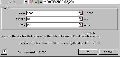
Type <Year> box 2000
Type <Month> box 2
Type <Day> box 29
Click Cell A11
Type Today is:
Click Cell B11
Click <Edit or => button at the Formula bar
Click <Function> button
Click <TODAY>
The Formula Palette appears.
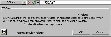
Click <OK>
Using the Formula Paste Functions
The Formula Paste Functions offers a third option of entering Formula. The Formula Palette lists each function and its arguments, a description of each function and its arguments, and the calculated result of each function and the overall formula.
Click <Sheet4>
Rename <Sheet4> to <Simple Paste Function>
Click Cell C11
Click <Edit or => button at the Formula bar
Click <Function> button
Click <SUM>
The Formula Palette appears.
The Sum function total cells C1:C10
Click <OK>
Click Cell C12
Click <Edit or => button at the Formula bar
Click <Function> button
Click <COUNT>
The Formula Palette appears.
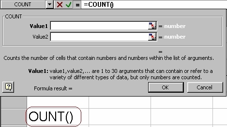
Click <Expand>
Select Cells C1:C10
The COUNT function counts cells C1:C10
Click <OK>
Click Cell C13 or C14 or C15 respectively
Click <Edit or => button at the Formula bar
Click <MAX> or <MIN> or <AVERAGE>
The Formula Palette appears.
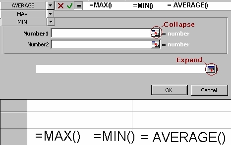
Click <Collapse> button at Number 1 box
Select C1:C10
Click <OK>
Auto Calculate
On the Status bar at the bottom of the screen, by position the mouse cursor with a right-mouse click, other function commands like Average, Count, Max, Min and Sum appear.
Using the COUNTIF (Range, Criteria)
Using the COUNTIF function to count the number of cells within a range which meets the given criteria.
Click Cell B17
Click <Edit or => button at the Formula bar
Click <Function> button
Click <COUNTIF>
The Formula Palette appears.
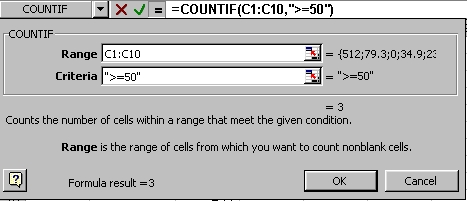
Click <Collapse> button at Number 1 box
Select C1:C10
Click at Number 2 box
Type ">=50"
Click <OK>
Using the IF Function
Using the IF function creates a conditional formula. The result of a conditional formula is determined by the state of a specific condition or the answer to a logical question.
The IF funcion requires the following syntax:
IF(Logical_test, Value_if_true, Value_if_false)
Logical test - expression to be evaluated as true or false
Value_if_true - value returned if the logical_test expression is true
Value_if_false - value returned if the logical_test expression is false
Click <Sheet5>
Rename <Sheet5> to <IF Example>
Use the IF Example at M3: Page 12
We will determine the PASSED or FAILED grading for the students.
Click Cell C2
Click <Paste function> button
Click <Logical>
Select <IF>
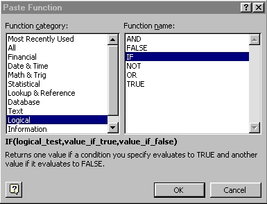
Click <OK>
Type B2<50 at the Logical Test box
Type "FAIL" at the Value_if_true box
Type True at the Value_if_false box

Click <OK>
Using the VLOOKUP Function
Using the function to search for a value in the leftmost column of a table, and then returns a value in the same row from a column you specify in the table.
=VLOOKUP(LOOKUP VALUE, COMPARE ARRAY, COLUMN INDEX)
Click <Sheet6>
Rename <Sheet6> to <Vlookup Example>
Use the VLOOKUP Example at M3: Page 14
Click Cell C7
Click <Paste function> button
Select <VLOOKUP>
Select B7 at the Lookup_value box
Select B1:C4 at the Table-array box
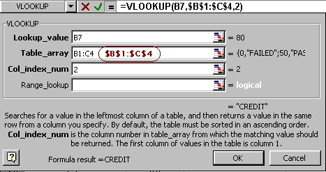
Edit $B$1:$C$4
Type 2 at the Col_index_num box
Click <OK>

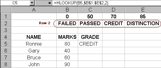
Using the HLOOKUP Function
Using the function to search for a value in the top row of a table or an array of values, and then returns a value in the same column from a row you specify in the table.
=HLOOKUP(LOOKUP VALUE, COMPARE ARRAY, ROW INDEX)
Click <Sheet7>
Rename <Sheet7> to <Hlookup Example>
Use the HLOOKUP Example at M3: Page 15
Click Cell C7
Click <Paste function> button
Select <HLOOKUP>
Select B5 at the Lookup_value box
Select B1:E2 at the Table-array box
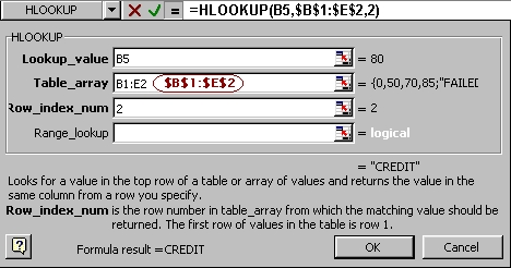
Edit $B$1:$E$2
Type 2 at the Row_index_num box
Click <OK>
Click <File> <Save>


Click
<File>
<Close>
Practice Exercises
Click <File>
<New>
<Save As>
My
Second Excel2000
at
<My Documents> folder
Practice
Exercise 1 :
M3:
Page 17
Click
<Sheet1>
Rename <Sheet1>
to <M3Ex1>
Practice
Exercise 2 :
M3:
Page 18
Click
<Sheet2>
Rename <Sheet2>
to <M3Ex2>
Practice
Exercise 3 :
M3:
Page 19
Click
<Sheet3>
Rename <Sheet3>
to <M3Ex3>
Practice
Exercise 4 :
M3:
Page 20
Click
<Sheet4>
Rename <Sheet4>
to <M3Ex4>
Click <File> <Close>
Click <File> <Exit>
Practice
Project 1
Practice
Excel
2000 Project1
Click <File> <Save>
Click <File> <Close>
Click <File> <Exit>
 Edwin
Koh : We
completed on the New
Knowledge and Skills in
Edwin
Koh : We
completed on the New
Knowledge and Skills in
Excel
2000 Module 3.